How to Use ISBETWEEN Function in Google Sheets

The ISBETWEEN function in Google Sheets is useful when you need to determine whether a given number is within a range of numbers or not.

For some reason, you may need to check if a number is between two other numbers. Even though this is just basic math, it may be time-consuming to do it in hundreds or thousands of numbers.

Wouldn’t it be great if you could automate it to speed things up? Well, you’ll be glad to know that the ISBETWEEN function does just that. The ISBETWEEN function in Google Sheets determines if a given value falls within the range of two values. In such a case, the return value is TRUE. Otherwise, it returns FALSE.

Here’s a practical example.

A nurse keeps a spreadsheet that serves as a daily monitoring system for the body temperature of patients. Let’s assume that the normal temperature for adults ranges from 36.1°C to 37.2°C. Through the ISBETWEEN function, the nurse can include a column showing whether each patient’s temperature is normal or not.

That is just one of the numerous use cases of ISBETWEEN function in Google Sheets. You will learn more about it as you go through this article. We’ll also look at how we can maximize it with other functions.

Let’s get started!

The Anatomy of the ISBETWEEN Function in Google Sheets

To utilize the ISBETWEEN function, let’s first understand its syntax. The function goes like this:

• = the equal sign indicates the beginning of a function. We type this whenever we want Google Sheets to perform a certain function.
• ISBETWEEN() this is our ISBETWEEN function.
• value_to_compare is our first parameter. This will hold the value we want to test if it’s within a range of two numbers.
• lower_value parameter should contain the start value for the range in which the value_to_compare can fall within.
• upper_value parameter should hold the range’s last value.
• [lower_value_is_inclusive] is an optional parameter that can hold TRUE or FALSE values. This parameter defines whether the lower_value should be included in the range or not.
• [upper_value_is_inclusive] on the other hand, holds the value that specifies whether upper_value is included in the range.
  

A Real Example of using ISBETWEEN Function in Google Sheets

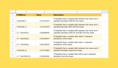
Below is an example that demonstrates how to use the ISBETWEEN function.

If we focus on the first two records, we only use the basic syntax of the ISBETWEEN function, that is, without the optional parameters [lower_value_is_inclusive] and [upper_value_is_inclusive]. By default, these parameters are set to TRUE, so you don’t have to indicate the value if you wish to include both the lower and upper values on the range.

In the case above, the ISBETWEEN function essentially answers the question, “Is the value provided within the specified range?”. This function returns either TRUE or FALSE values.

What happens when we override the optional parameters?

Taking a look at the last record, the Value to Compare in the last row is the same as the last value of the range, which is 250. Since we specified the last parameter (upper_value_is_inclusive) as FALSE, we are basically instructing the function to exclude 250 in the range. As a result, we get a FALSE result.

Do you see how easy that is? If you would like to have a copy of my example spreadsheet, go ahead and click the link below.

Make a copy of the example spreadsheet

Now, let’s try to utilize the ISBETWEEN function in a real-world setting.

How to Use the ISBETWEEN Function in Google Sheets

We’ll use the scenario earlier about the body temperature monitoring system for this activity. Our objective is to use the ISBETWEEN function to determine whether each patient’s body temperature is normal or not, based on the notion that normal temperature is within 36.1℃ to 37.2℃.

1. Start by creating a copy of the example spreadsheet through the link above. Once you make a copy, navigate to Sheet2.
   
   
   
   
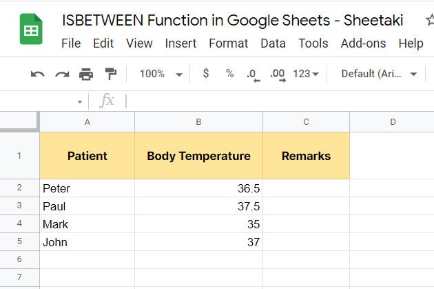
2. We need to fill in the Remarks column to complete the report. Let’s start with Peter’s record. Double-click cell C2 and type in the equal sign ‘=’ followed by ‘ISBETWEEN(‘ to initiate the function.
   
   
   
   
3. Next, we need to specify the parameters of our ISBETWEEN function. For our first parameter, we need to use the cell reference of Peter’s body temperature, which is B2. Type in ‘B2’ as the value of our value_to_compare parameter.
   
   
   
   
4. The next two parameters define the range of numbers between which we want to test whether the value_to_compare exists. Indicate ‘36.1’ as the lower_value and ‘37.2’ as our upper_value.
   
   
   
5. At this point, we can already set the optional parameters. In our case, though, we need to include the values of both the lower_value and upper_value parameters on the range. It was mentioned previously that the optional parameters are set to TRUE by default, so it’s fine to leave them out in this case.
   
   
   We now just need to complete the function by typing in the close parenthesis ‘)’. Afterward, hit the Enter key on your keyboard to display the result.
   
   
   
   
6. Now, use the autofill feature to complete the series. Just select cell C2 and drag the small blue box on its lower right corner towards the rest of the records.
   
   
   
   

Great job! We just identified who among the patients has a normal temperature just by using the ISBETWEEN function. However, it’s somewhat inappropriate to use TRUE or FALSE values as the remarks, isn’t it?

Fortunately, Google Sheets lets you combine functions, allowing you to format your report in a more readable way.

Combining the ISBETWEEN Function With Other Function

In our previous example, we successfully used the ISBETWEEN function to determine whether a temperature result was normal. The drawback of this function is that it doesn’t allow us to edit the value that it will return once the condition is true or not. So, we’re just stuck with two return values, TRUE or FALSE.

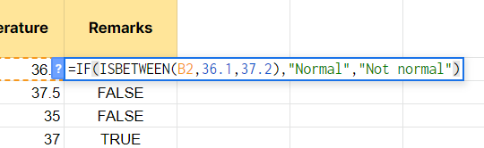
Suppose we want the remarks column to display “Normal” or “Not normal”, we can edit the formula to include an IF function. Just follow the steps below.

1. With the spreadsheet still open, double-click cell C2 to enter edit mode.
   
   
   
   
2. Right after the equal sign ‘=’, type in ‘IF(’. This will now make the entire ISBETWEEN function the first parameter of the IF function.
   
   
   
   
3. For the next two parameters, indicate ‘Normal’ and ‘Not normal’ respectively. Be guided by the image below.
   
   
4. Finish the formula by pressing the Enter key on your keyboard and use the autofill feature to complete the rest of the remarks. Your spreadsheet should now look like this:
   
   
   
   

Perfect! You just learned how to combine the ISBETWEEN with another function. If you would like to know more about the IF Function, make sure to check out this article.

That’s pretty much it when it comes to using the ISBETWEEN function. Well done! You just learned how to write its basic syntax and how to use it with another function in Google Sheets.

Be the first to know more about other useful content like this article by subscribing to our newsletter.