


The ISOWEEKNUM function in Google Sheets is useful for finding out what week a specific date falls into.
Table of Contents
In dealing with financial reports, it will likely be necessary to determine what week of the year a certain transaction falls into. A calendar is always at your fingertips, but it takes some effort to identify the week of a particular date. It’s here where the ISOWEEKNUM function comes in handy.
As the name suggests, ISOWEEKNUM returns the week number of a date in accordance with the ISO standard, which is ISO 8601.
Following this standard, weeks are counted starting from Monday to Sunday. The numbering of weeks starts from the first week of the year that contains a Thursday. As an example, the first week of the year 2021 is from January 4 to January 10. So, when we use the ISOWEEKNUM for the date January 5, 2021, the function returns 1 as the result.
The Anatomy of the ISOWEEKNUM Function
ISOWEEKNUM is one of the simplest functions in Google Sheets. To use it in your spreadsheets, you just need to follow this syntax:
As you can see, the syntax is quite self-explanatory. Here’s the breakdown of the components:
- = we use the equal sign to indicate our intention of writing a function or formula.
- ISOWEEKNUM() this is our
ISOWEEKNUMfunction. - date is the only parameter that the function requires. It should contain a date, number, or another function that returns a date value.
A Real Example of Using ISOWEEKNUM Function
Let’s consider a simple use case for the ISOWEEKNUM function.
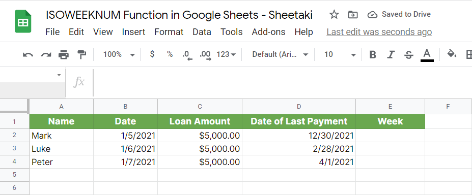
Every first week of the year, John offers a $5,000 loan payable in 1 year. He records each transaction in a spreadsheet that serves as his monitoring system to keep track of the loans. Here is a screenshot of his spreadsheet.

John has a unique formula for computing the loan interests. However, to make it work, he must determine what week each borrower’s last payment falls on. So, in his spreadsheet, he assigned another column and used the ISOWEEKNUM function to do the job.

Now, John doesn’t need to scan through his calendar just to determine the week number of each last payment record.
You can make a copy of the example data if you want to play with the ISOWEEKNUM function. Just click the link below.
ISOWEEKNUM seems pretty straightforward, right? Now, let us learn how to write this function properly.How to Use ISOWEEKNUM Function in Google Sheets
- First, open the spreadsheet that you intend to use the
ISOWEEKNUMfunction to. If you don’t have one at the moment, you can make a copy of our example spreadsheet earlier.
- Upon opening the spreadsheet, double-click the cell where you need to enter the function. In our example below, cell E2 is selected.
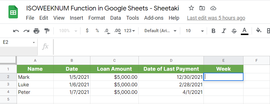
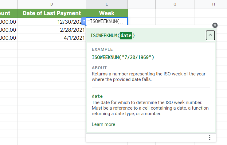
- Next, type in the equal sign ‘=’, followed by ‘ISOWEEKNUM(’ to start our function.
- Now that you have initiated the function, specify its date parameter. In our case below, we indicated the cell reference of the last payment date (D2) as the parameter.
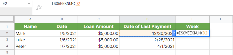
- At this point, close the function by typing in the close parenthesis ‘)’ Afterward, press the Enter key on your keyboard to show the result.

- If you need to recreate the formula in adjacent cells, you can always use the autofill feature of Google Sheets. Just select the cell that contains the function, then click and drag the small blue box on the lower right corner over the cells where you want to paste the formula.

That’s how you write a basic ISOWEEKNUM function in Google Sheets. In addition to this, you can also use a function as the parameter of ISOWEEKNUM. Learn how to do it in the next section.
Using the ISOWEEKNUM Function in Google Sheets with Another Function
You can also use another function as the parameter of ISOWEEKNUM, provided that the function returns a date data type. Let’s try this simple activity to test this use case.
- Start a new Google Sheets spreadsheet or use the one from the previous activity.
- Double-click any cell where you want to enter the function. Cell A1 is selected in the example below.
- This time, initiate the function by typing in ‘=ISOWEEKNUM(’.
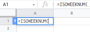
- Our objective for this activity is to return the week number of the current date. For this to work, we need to use the NOW() function. If you are not aware yet, this function returns the current date. At this point, type in ‘NOW()’ as the parameter of the
ISOWEEKNUMfunction.

- Lastly, hit enter on your keyboard to display the result.

This article was written on October 20, 2021, so the return value is 42.
Well done! Now you know how to write the ISOWEEKNUM in Google Sheets. Take note, however, that there are certain things that you need to consider when using this function.
Points to Consider When Using the ISOWEEKNUM Function in Google Sheets
- If you need to enter the actual date instead of a cell reference as the parameter, you need to use the DATE function. If you fail to do so, the function might return an error.

- You can also specify the actual date as the parameter without using a function. You just need to enclose the date in double quotation marks and follow the format mm/dd/yyyy or yyyy/mm/dd.

- In compliance with ISO 8601, the first week of the year is the week that contains the first Thursday. As a result, if you use the function for a date before the first week is counted, it returns either 52 or 53.
That’s about it when it comes to using the ISOWEEKNUM function in Google Sheets. Now you know how to write its syntax and combine it with another function to make your work more efficient.
Check out also our other articles in Google Sheets for you to master this powerful spreadsheet program.
Make sure to subscribe to our newsletter to get more useful Google Sheets content like this article.


