How to Use LEFT Function in Google Sheets

The LEFT function in Google Sheets is useful to return a substring from the beginning of a specified string.

The LEFT function is one of the text functions that let you format your text values (strings) in Google Sheets.

Let’s take an example.

Say you have product codes of clothes that contain several numbers, letters and special characters.

To get the category of products, you need to cut the beginning of the text values until the first ‘_’ underscore character.

So how do we do that?

It’s pretty simple.

The LEFT function just needs an input string and the length of the substring to extract it.

Let’s dive right into some examples to see how we can write our own LEFT function in Google Sheets.

The Anatomy of the LEFT Function

The syntax of the function defines how we should work with it. The syntax of the LEFT function is as follows:

=LEFT(string, [number_of_characters])

Let’s understand what the LEFT function and its attributes mean:

• = the equal sign is how we start just about any function in Google Sheets.
• LEFT is our function. We will have to add the corresponding arguments string (required) and number_of_characters (optional) into it for it to work.
• string is the input text from which the function returns the left part.
• number_of_characters is an optional argument. It specifies the number of characters to return from the left side of the text. Its default value is 1, so in case the number is not specified, the function returns the single leftmost character in the string.

A Real Example of Using LEFT Function

Let’s look at the example below to see how to use the LEFT function in Google Sheets.

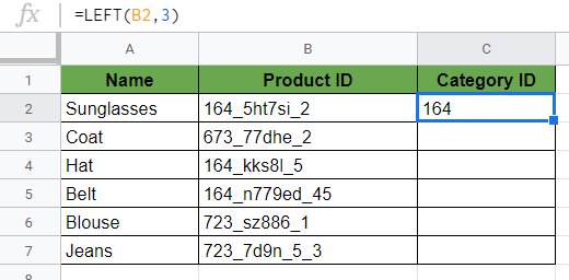
This sheet contains a list of products, and each product has a long identification code that we call Product ID in column B.

Our task is to extract the left side of these IDs until the first underscore and write it as Category ID in column C.

LEFT Function With Static Number of Characters

In the example above, it’s pretty simple. If you look at the sheet, you can see that the Product IDs always have 3 numeric characters on the left side of the first underscore symbol.

So we use a static (non-changing) value to extract the left part of the strings.

The following formula will extract the first three characters of the cell content of B2:

=LEFT(B2, 3)

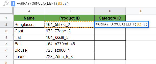
However, we want to apply the same formula to all of the products in the sheet, not only the first one.

• One option to do write (or drag down) the same function into all of the cells of column C.
• Another way is to use the ARRAYFORMULA function. If you want to know more about how to use ARRAYFORMULA function in Google Sheets, check out our article on that.

So, we can add the ARRAYFORMULA to our LEFT function as follows:

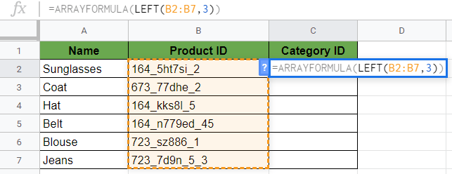
=ARRAYFORMULA(LEFT(B2:B,3))

Here’s what this example does:

• The LEFT function has two arguments. The first one is the text value we want to use, so the string argument. These text values are present in column B from cell B2 to cell B7. Therefore we wrote B2:B7.
• The second argument of the LEFT function is the number_of_characters, which is 3 in our example.
• We used the ARRAYFORMULA function to apply the function to the whole array of products.

It’s simple, isn’t it?

LEFT Function With Dynamic Number of Characters

Let’s change the Product IDs to see how to use the LEFT function in a little bit more complicated example.

We don’t want to extract the first three numeric characters anymore, but we need numbers of different lengths before the first underscore symbol.

So what can we do now?

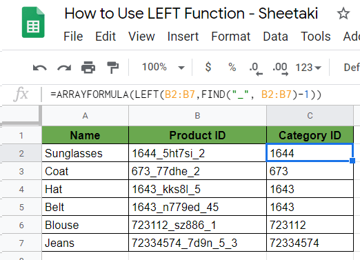
We can use the FIND function additionally. The FIND function in Google Sheets is used to return the position at which a string is first found within the text.

This way, we look for the first underscore characters dynamically.

The function to put in cell C2 is as follows:

=ARRAYFORMULA(LEFT(B2:B7,FIND("_", B2:B7)-1))

Let’s see what happens here:

• As before, we use the LEFT function with two arguments. The first argument (string) doesn’t change. It’s still the range B2:B7 where the original string values are.
• The second argument is the whole FIND formula: FIND(“_”, B2:B7)-1.
• We started with the name of the FIND function followed by the character we want to find. This character is the “_” underscore character, and we had to put it between quotation marks.
• Then we added the range of cells where we are looking for the specified character. The range is the same B2:B7 where our text values are.
• After that, we subtracted 1. We needed this –1 because the FIND function gives us the position of the first underscore character. However, we want to extract the substrings before that character, so we subtract one. For example, if the underscore is the 5th character in a string, then we need the first four characters of the string.
• We used the ARRAYFORMULA to apply the function to the whole list of products. As a result, we extracted the numeric characters from the beginning of the strings, even though their lengths are different.

You can make a copy of the spreadsheet below and try it for yourself:

How to Use LEFT Function in Google Sheets

Let’s see how to write your own LEFT function, step-by-step.

1. To start, click on the cell where you want to show your result to make it the active cell. For this guide, I will be selecting C2, where I extracted the first substring.

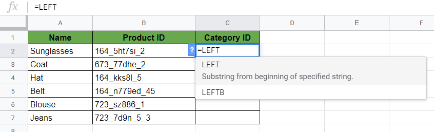
2. Next, type the equal sign ‘=’ to begin the function. Then followed by the name of the function which is ‘left‘ (or LEFT, whichever works).

3. Now you should see that the auto-suggest box will pop-up with the name of the functions that start with LEFT. There are more of them, so make sure to select the right one!

4. After the opening bracket ‘(‘, you have to add the right arguments. Firstly, highlight the cell that has the original text value. In my example, I click on the cell B2.

5. After that, add a comma to separate the values and write the required number_of_characters you want to return from the left side of your string. I’m writing 3 here to extract the first three characters of my string.

6. Now you can hit your Enter key to get the result of this single product immediately.

7. Let’s see how should you apply the function to the whole list of products using ARRAYFORMULA. To make it work, type ARRAYFORMULA at the beginning of the whole function after the ‘=’ equal sign and then add the ‘(‘ opening bracket.

8. When working with ARRAYFORMULA, you also need to change the cell references to ranges of cell references. So, instead of using B2 as the text argument, change it to the whole range of cells, to B2:B7 in my example.

9. Close the brackets and hit Enter! You can see your results in the whole array.

That’s it, well done! You can now use the LEFT function together with the other numerous Google Sheets formulas to create even more powerful formulas that can make your life much easier. 🙂

Get emails from us about Google Sheets.

Our goal this year is to create lots of rich, bite-sized tutorials for Google Sheets users like you. If you liked this one, you'll love what we are working on! Readers receive ✨ early access ✨ to new content.

Subscribe