How to Use RIGHT Function in Google Sheets

The RIGHT function in Google Sheets is useful to return a substring from the end of a string.

The RIGHT function extracts a specific number of characters from the right side of a text value and returns that fraction.

Let’s take an example.

Sometimes you don’t need the whole content of a cell, but you just want to extract the last characters of cell content.

For example, when you work with URLs, you might want to cut off the “https://” from the beginning of them. 🔗

So how do we do that?

Simple.

To do so, use the RIGHT formula with just an input string and the length of the substring that you want to return from the right side of the text.

Let’s dive into the examples below, where we will deal with actual values and see how we can write our own RIGHT function in Google Sheets.

The Anatomy of the RIGHT Function

The syntax of the function defines how we should work with it. So the syntax (how we write) the RIGHT function is as follows:

=RIGHT(string, [number_of_characters])

Let’s understand what the RIGHT function and its attributes mean:

• = the equal sign is how we start just about any function in Google Sheets.
• RIGHT is our function. We will have to add the arguments string (required) and number_of_characters (optional) into it for it to work.
• string is the input text from which the function returns the right part.
• number_of_characters is an optional argument that specifies the number of characters to return from the right side of the text. The default value is 1, so if you don’t specify this number, the function returns the last single character of the text.

⚠️ A Few Notes to Make Your RIGHT Function Work Perfectly

1. In case the number_of_characters is greater than or equal to the length of the original text, then the function returns the original source string.
2. The number_of_characters argument must be greater than or equal to 1.
3. In addition, if you ignore the second argument, then only the one last character will be extracted.
4. The RIGHT function has an opposite function which is the LEFT function. Similarly, the LEFT function returns a substring but from the left side of a text value instead of the right side.  Read our previous article on How to Use LEFT Function in Google Sheets guide so you can clearly see the difference.

A Real Example of Using RIGHT Function

Let’s look at the example below to see how to use the RIGHT function in Google Sheets.

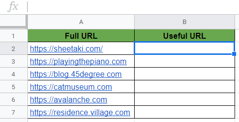
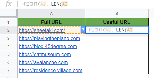
In the example above, we have a list of URLs, and originally they have “https://” at the beginning. This is column A with the full URLs.

For this guide, we will be removing these parts from the URLs and only keep the right side of them. We want to extract these useful URLs in column B.

As I have shown, the RIGHT function needs two arguments: (1) the text you want to cut and (2) the number of characters you want to keep on the right side of the text.

However, we don’t have an exact number of characters we want to extract here. We only know how many characters we don’t need from the beginning of the URLs.

We need to calculate it with the use of other functions. That will be the LEN function that counts the total number of characters of a string.

So we want to calculate the number of characters that we want to keep from the right side of the text values. To do this, we count the total number of characters and then subtract the number of characters we don’t need.

Accordingly, the RIGHT formula we used in cell B2 is as follows:

=RIGHT(A2, LEN(A2)-8)

Here’s what this function does:

• To start, we have actively selected the cell B2 where we want to write our formula. This is where we want to use the RIGHT function to return the substring from the right side of the URL.
• We selected cell A2 that serves as our string argument containing the original text.
• Secondly, we calculated number_of_characters according to the length of the whole string and the length of “https://” that we want to cut off.
• To do this, we used the LEN function to get the total number of characters. We simply added one cell reference into it to count the characters in cell A2.
• We subtracted 8 because “https://” has precisely eight characters. This way, we ensure that the second argument of the RIGHT function is the length of the whole text minus the length of “https://”.
• The RIGHT function returns the right side of the string without the first 8 characters.
• Finally, we applied the same function with the corresponding references to every URLs in the sheet.

Super easy, right?

You can try it by yourself by making a copy of the spreadsheet using the link I have attached below:

How to Use RIGHT Function in Google Sheets

Let’s begin writing our own RIGHT function in Google Sheets.

1. To begin, click on the cell where you want to show your result to make it the active cell. For this guide, I will be selecting B2, where I wanted to extract the first useful URL.

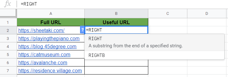
2. Next, type the equal sign ‘=’ to begin the function and then followed by the name of the function which is ‘right‘ (or ‘RIGHT‘).

3. Now you should see that the auto-suggest box will pop-up with the name of the functions that start with RIGHT. Make sure to select the right one, because there are more of them!

4. After the opening bracket ‘(‘, you add the variables. The first variable is the string you want to cut. You can reference a cell or type your text directly between quotation marks. I’m using the cell reference A2 by simply clicking on it.

5. Then, add a comma to separate the arguments. After that, you can write your formula that calculates number_of_characters. It can be a number or a more complicated formula. For this example, use the LEN function to get the total number of characters. So start writing its name and select it from the auto-suggest box.

6. Afterwards, click on the cell that has the original text to add it as the argument of the LEN function. For this guide, I will be clicking at cell A2 again. Type the ‘)‘ closing bracket.

7. Then, you should think about how many characters do you want to cut off from the string. You start with the total number of characters, and you should subtract the number of unnecessary characters. In this example, “https://” has eight characters. With this in mind, I’m subtracting 8 from the length of the full URL.

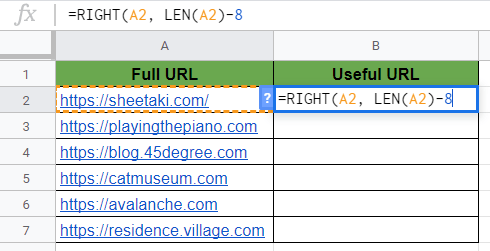
8. Press the Enter key to add the closing brackets ‘)‘ and to complete the function. As a result, you can see the substring without “https://” in cell B2.

9. Drag down the function with your mouse to apply it to the whole list of URLs. You can do this by clicking on the little blue square in the bottom right corner of the cell.

That’s pretty much it to using the RIGHT function in Google Sheets. Feel free to go through the other numerous Google Sheets formulas to create even more powerful formulas that can make your life much easier. 🙂

Get emails from us about Google Sheets.

Our goal this year is to create lots of rich, bite-sized tutorials for Google Sheets users like you. If you liked this one, you'll love what we are working on! Readers receive ✨ early access ✨ to new content.

Subscribe