This guide will explain how to create your own order tracker sheet in Google Sheets.
We will show how to set up an order database and a separate sheet for clients to view order status.
Let’s take a look at a simple example of a use case where an order tracker might be necessary.
Suppose you are a freelance artist that accepts custom requests. Using a Google Form, you’ve collected data on the type of art they want, their contact details, and the shipping address.
Results from the Google Form are placed in a Google Sheet spreadsheet automatically. Since you want to keep track of each of these orders, you’ve added additional columns to indicate the order status. For example, you can indicate that the work is either ‘In Queue’, ‘ In Progress’, or ‘Shipped’.
How can we let the client know the progress of their request without having to show the entire order tracker?
This guide will show how you can use the VLOOKUP function and built-in protection options to create a client-side tracker that keeps your data safe.
Let’s take a look at how an order tracker sheet looks like on an actual spreadsheet in Google Sheets.
A Real Example of an Order Tracker Sheet in Google Sheets
Let’s take a look at a real example of an order tracker sheet in a Google Sheets spreadsheet.
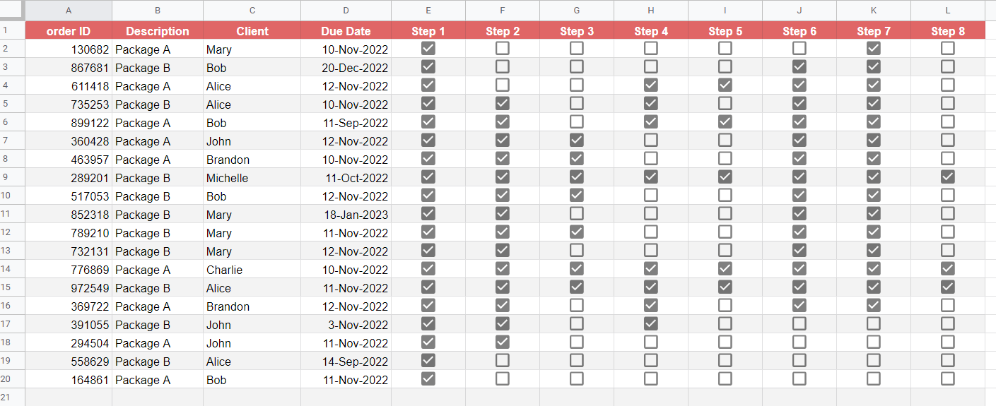
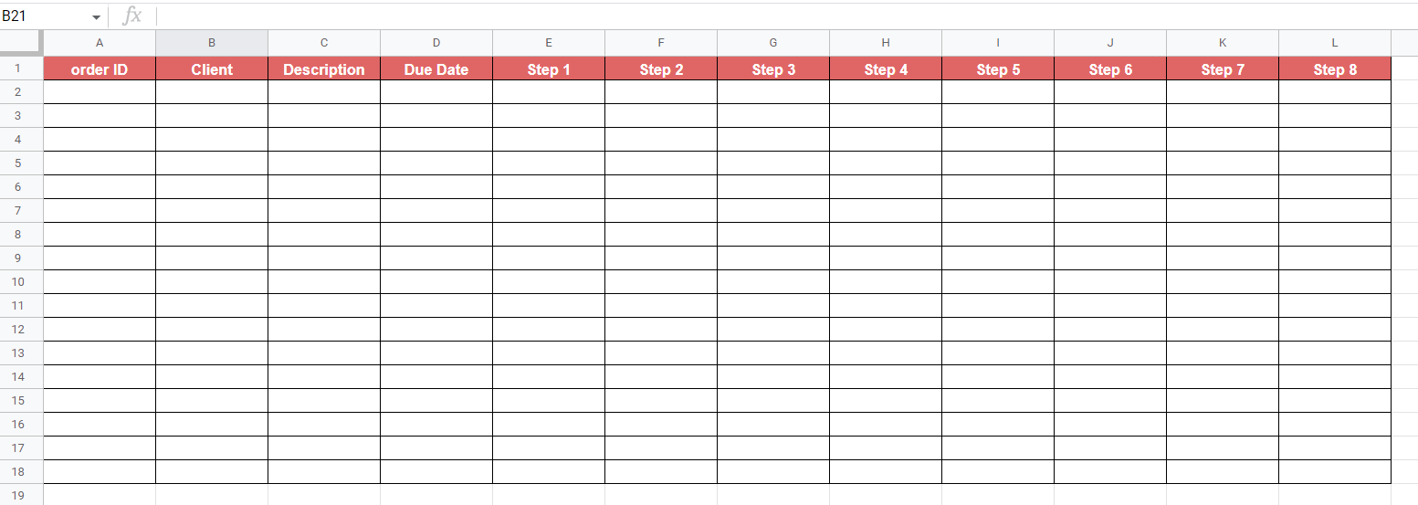
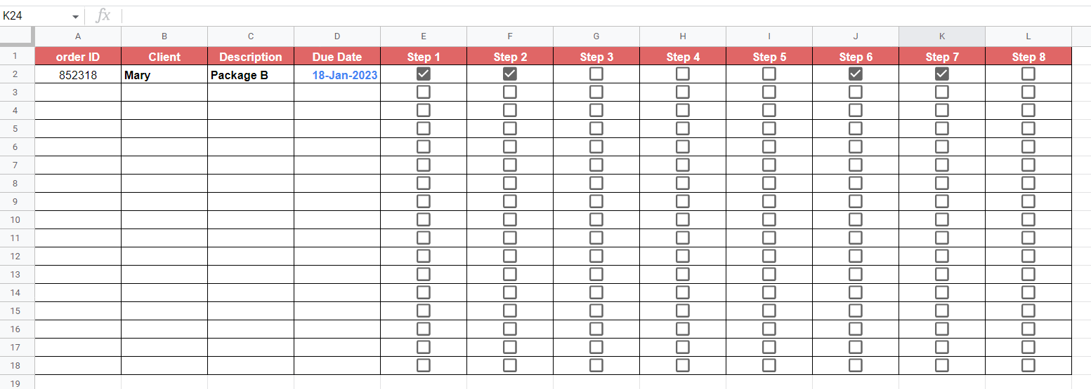
The spreadsheet seen below includes order data such as the order ID, order description, client name, and due date. The table also includes additional columns indicating whether a particular process step has been accomplished.
![]()
This is a general format that we can apply to various use cases. For example, if each order was a custom T-shirt, step 1 could be the initial drafting stage. Afterwards, we can have a ‘For Printing’ status, a ‘Shipping’ status, and an ‘Ordered’ Status.
If the client requests the order status, it might be unwise to send the original database. To help facilitate the order tracking, we can make a tracker that looks up data from our original table. The client simply needs to provide the order IDs to populate their copy of the tracker.
![]()
To get the values in Column B, we just need to use the following formula:
=IFNA(VLOOKUP($A2,'Order Database'!$A$2:$L$20,3,FALSE),"")
We use the VLOOKUP function to look up values corresponding to column A’s order IDs. We wrap the function with an IFNA function in case no matches are found.
You can make your own copy of the spreadsheet above using the link attached below.
If you’re ready to try out the VLOOKUP function yourself, follow our guide on creating an order tracker sheet in Google Sheets.
How to Create an Order Tracker Sheet in Google Sheets
This section will guide you through each step needed to set up an order tracker sheet in Google Sheets. You’ll learn how we can refer to the tracker sheet to create a table that clients can use to determine the status of their orders.
Follow these steps to create an order tracker sheet in Google Sheets:
- First, we’ll need to set up the main order tracker sheet. The fields to include in this table will depend on your use case but usually includes a unique order ID and one or more columns indicating the order status.
 In the sample database above, we’ve added checkboxes for each step to make it easier for the spreadsheet owner to update the status of each order.
 - Next, we’ll create a new sheet that will only be accessible to a particular client. We can copy the same headers from the original database.
- Once we have our table set up, we must now fill it with the appropriate data. Since column A is reserved for user input, we’ll start filling up the Client column using our
VLOOKUPformula.
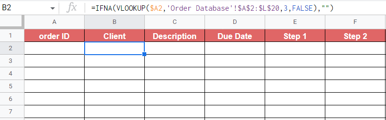
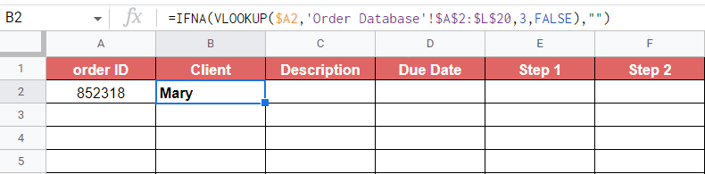
- If the client inputs a valid order ID, the formula should output the corresponding data from the original tracker.
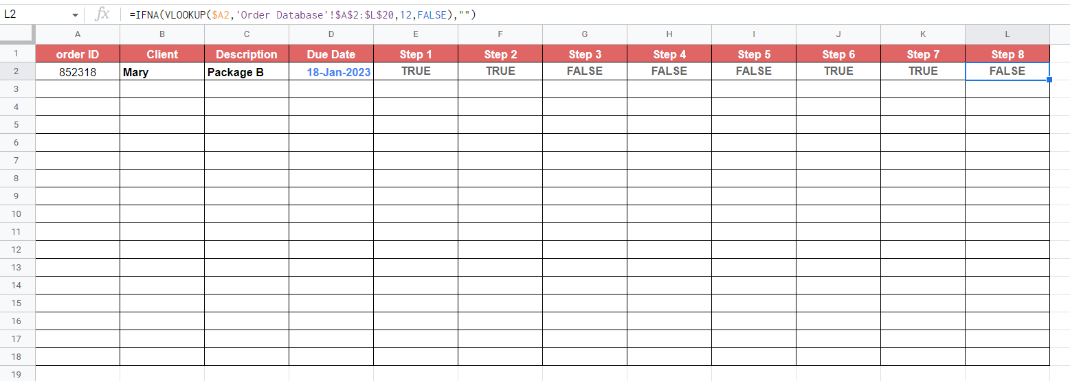
- Copy the formula on the first cell of the remaining columns. We can use the Fill Handle tool to perform this quickly with a simple drag to the right. The only argument we need to change for each formula is the column number.
- To add checkboxes to the client sheet, select the range of cells you want to convert to checkboxes and click on the Checkbox option under the Insert menu.
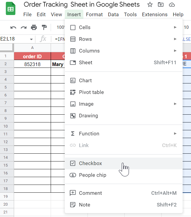
- Once checkboxes have been added, cells with a value of TRUE are represented with a checked checkbox.
- Use the Fill Handle tool to add the
VLOOKUPformula to the rest of the rows.

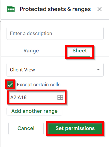
- Since we want to prevent clients from editing cells with formulas, we must add protection to our spreadsheet. Click on the Protect sheets and ranges option under the Data tab.

- In the Protected sheets & ranges panel, navigate to the Sheet tab. Check the option labeled ‘ Except certain cells’ and place the range you want the client to have access to. Click on the Set permissions button to set the specified protection.
This step-by-step guide should be all you need to create an order tracker sheet in Google Sheets. Our tutorial shows how you can add checkboxes to your order tracker to quickly update your orders’ status.
We’ve also shown how to create a client-side tracker using VLOOKUP. This additional sheet lets your clients see their order status by providing their unique order ID.
The VLOOKUP function is just one of many functions you can use to filter data you need in Google Sheets. With so many other functions available, you can surely find one that suits your use case.
Are you interested in learning more about what Google Sheets can do? Subscribe to our newsletter to find out about the latest Google Sheets guides and tutorials from us.