Creating named ranges in Google Sheets allows you to recall and reuse groups of cells more efficiently.
Table of Contents
Most of the time, you’ll need to use cell ranges for your formulas in Google Sheets, so keeping track of these ranges is helpful. However, calling on the same cell range across different parts of your spreadsheet could be very inconvenient. This is where creating named ranges can benefit you.
As we all know, cells in Google Sheets have their own addresses, and we use them as identifiers. The same concept applies to named ranges, but we are dealing with cell ranges instead. When you create a name for a particular range of cells, you can use it whenever you need to include that cell range in your calculations.
In this guide, you’ll learn the benefits of creating named ranges in Google Sheets and how to set them up.
Let’s get right to them!
Why Should you Create Named Ranges in Google Sheets
You could argue that cell ranges already have their own addresses, and they already serve the purpose of named ranges. So, why do you still need to create named ranges? Well, here are two great reasons why you need to name your cell ranges in Google Sheets:
- Creating a named range allows you to assign a descriptive name for a range of cells and use it in your formulas. For instance, you can just write the formula ‘=AVERAGE(GradesData)’, rather than ‘AVERAGE(C2:C11)’. This makes it easier for you to recall the cell range each time you need it.
- Named ranges save you a significant amount of time and effort. Let’s say you use a particular named range for different formulas in your spreadsheet. If you update the data range of your named range, the formulas that use it will automatically refer to the new range.
As you’ve read, named ranges will help you deal with cell ranges more efficiently. They can help simplify your complex formulas, so it’s a great advantage if you know how to create and use one.
How to Create Named Ranges in Google Sheets
This time, let’s learn how to create a named range in Google Sheets. Click the link below to generate a copy of our example spreadsheet so you can follow along.
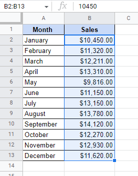
- The spreadsheet contains a dataset of the monthly sales of a company. Our goal is to create a named range for the cell range that contains the monthly sales records. After that, we’ll use the named range to fill in the required fields in the spreadsheet: Average Monthly Sales, Lowest Sales, and Highest Sales.

- Start by highlighting the B2:B13 cell range, which contains the monthly sales.
- Next, click the Data menu and then choose Named ranges.

Upon clicking, the Named ranges panel will appear on your screen.
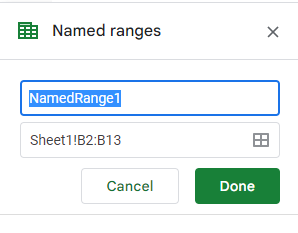
- From the Named ranges panel, type ‘SalesData’ as the name of our new named range into the first field. Afterward, make sure that the second field contains the cell range we have selected earlier (B2:B13), as shown in the image below:

- To save our new named range, simply click Done on the Named ranges panel.
We now have our named range for our monthly sales record. In the next section, you’ll learn how to utilize it in the spreadsheet.
How to Use Named Ranges in Google Sheets
Earlier, we created a named range called SalesData. Now, let’s use this named range in the different formulas that we’ll use to determine the average, lowest, and highest monthly sales.
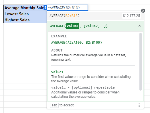
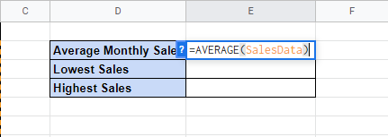
- Let’s start with the average monthly sales. To find out the average value of a numerical dataset, we just need to use the AVERAGE function. Begin by initiating the
AVERAGEfunction in cell E2. Type in the equal sign ‘=’, followed by the word ‘AVERAGE(’.
As you type in the function, you’ll notice that Google Sheets will recommend the cell range you can use for the current function. We will skip the recommendation for now since our goal is to use a named range.
- For the parameter of our
AVERAGEfunction, specify the named range we created earlier, SalesData. Make sure to close the formula by typing close parenthesis ‘)’.
 Then, press the Enter key on your keyboard to compute the average.

Great! You see how a named range works? Instead of using the cell range, you can just use its name to simplify your formulas.
- This time, use the MIN and MAX functions to determine the lowest and highest sales within the SalesData named range. Be guided by the image below.

If your formulas are correct, you should have the following results:

Good job! Now you know how to create and use named ranges in Google Sheets.
Naming Rules of Named Ranges in Google Sheets
You’ve seen how easy it is to create a named range in Google Sheets. However, you need to observe the following rules when naming a named range to prevent errors or issues:
- A named range can’t start with any number. So, it’s invalid to have ‘1SalesData’ as a named range.
- A named range can not be a cell reference like, ‘A2’, ‘D15’, or ‘B2:D7’.
- It can’t contain spaces or punctuation marks except for the underscore symbol ‘_’. For example, you can’t name a cell range ‘Grades Data’, but you can name it as ‘GradesData’ or ‘Grades_Data’.
- It should not exceed 250 characters.
That’s all there is to creating named ranges in Google Sheets. This technique may be useful when you have to repeatedly use the same cell range across multiple operations in your spreadsheet.
Check out our other articles in Google Sheets if you want to learn more spreadsheet skills.
Subscribe to our newsletter so you can be updated with other essentials in Google Sheets.