How to Use DPRODUCT Function in Google Sheets

The DPRODUCT function in Google Sheets is useful if you need to multiply the values in a field (column) of records in a list or database that matches the conditions that you specify.

The DPRODUCT function is a built-in function that is categorized as a ‘Database Function’. It can be used as a worksheet function, and can be entered as part of a formula in a worksheet cell.

Let’s take an example.

I am evaluating my trading strategies for this month and have listed the number of units purchased, and purchase value for each crypto coin. My need is to check net spend on Ethereum coins to calculate the profit/loss realized. To go through my entire portfolio for the same is a slightly time-consuming task.

And here is where DPRODUCT comes to my rescue. The function helps me calculate the product of units purchased and the cost incurred to give the total money spent on Ethereum coins.

That’s just one small example. There are plenty of other use-cases for this function in real life. 

Great! Let’s dive right into real-business use-cases, where we will deal with actual values and as well as learn how we can write our own DPRODUCT function in Google Sheets to calculate variances in data.

The Anatomy of the DPRODUCT Function

So the syntax (the way we write) of the DPRODUCT function is as follows:

=DPRODUCT(database, field, criteria)

Let’s dissect this thing and understand what each of the terms means:

• = the equal sign is just how we start any function in Google Sheets.
• DPRODUCT() is our DPRODUCT function. DPRODUCT will return the variance of an entire population selected from a database table-like array or range using a SQL-like query.
• database refers to the array or range having the data, including headers for each column’s values
• field refers to the column in the data which has the values that are to be extracted and worked on.
  • field may either be a text label referring to the required column header or a numeric value indicating which column to consider, where the first column has a value = 1.
• criteria refers to an array or range containing the criteria to filter the database values before operating. This may be left blank.

A Real Example of Using DPRODUCT Function

Take a look at the example below to see how DPRODUCT functions are used in Google Sheets:

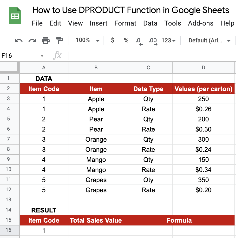
The above figures are pricing details for fruits in my state. The objective here is to find the price for 250 apples (which is equivalent to 1 carton at the store I am obtaining the data from). Just below the captured data, I have given a provision to enter the criteria (column A16) based on which the data will be filtered.

As you can see below, I have obtained the total price for 250 apples using the DPRODUCT function:

You may try changing the criteria and see how the result changes. Go ahead and make a copy of the spreadsheet using the link I have attached below:

Awesome! Let’s begin our DPRODUCT function in Google Sheets.

How to Use DPRODUCT Function in Google Sheets

1. Let’s see how to write your own DPRODUCT function, step-by-step. I have listed down the packaged food consumption of two kids from my neighborhood – Mike and Jamie, in the past year. The objective is to identify the total amount Mike spent on bars in the month of May. You will notice that I am using multiple conditions here.

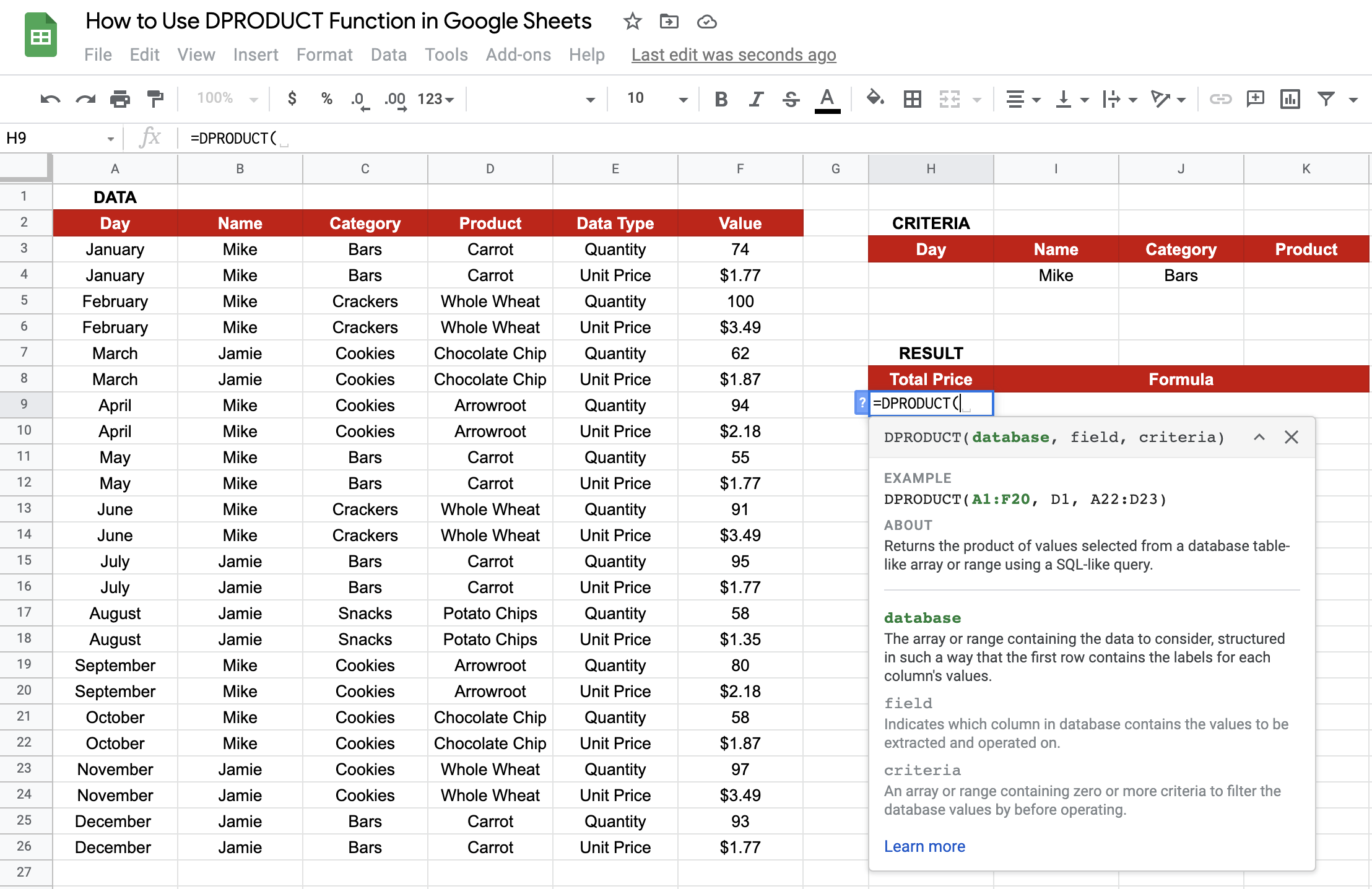
2. Now, simply click on any cell to make it the active cell. For this guide, I will be selecting H9, where I want to show my results.
3. Next, simply type the equal sign ‘=‘ to begin the function and then follow the function’s name, which is our ‘dproduct‘ (or DPRODUCT, whichever works).
4. You should find that the auto-suggest box appears with our function of interest. Continue by entering the first opening bracket ‘(‘. If you get a huge box with text in it, simply hit the arrow in the top-right-hand corner of the box to minimize it. You should now see it as follows:

5. Now, the fun begins! Let’s give the required inputs to the function to get the total price for bars that Mike purchased, per the filtration criteria we have given besides the data:

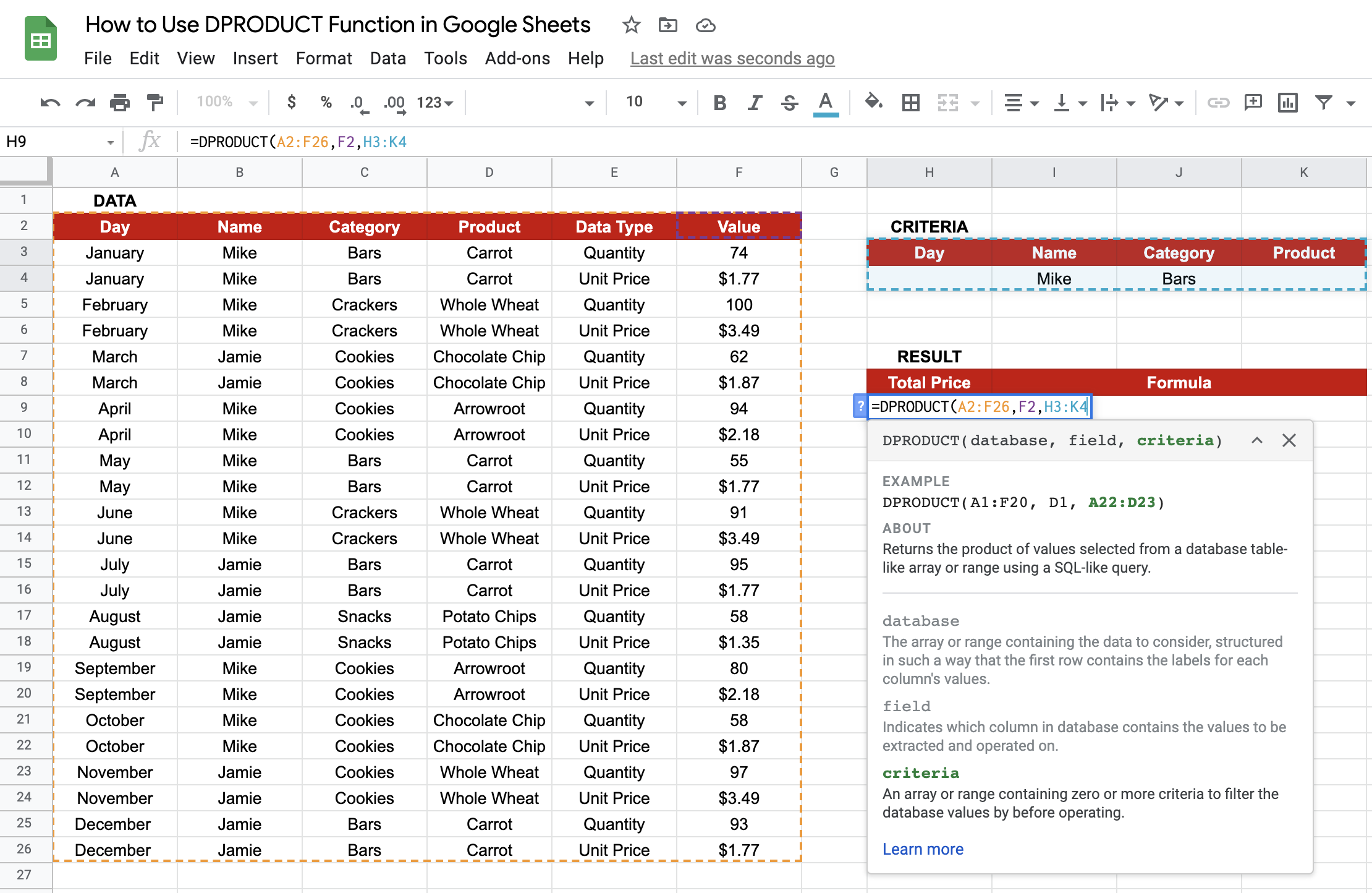
6. Take note of how I’ve specified conditions to limit the purchases to the ones Mike made on bars. The criteria for the formula are input as H3:K4 to account for all the criteria mentioned, if any.
7. Once you’ve entered the necessary database, field, and criterion values, or you’ve done what I did, make sure to close the brackets ‘)’, as shown below.

8. Finally, just hit your Enter key. You will notice that the result reads $12750.90. 

Fix Error in DPRODUCT Output

You are getting a high value as output because, based on the conditions you have given, the table gets filtered for four rows, two in January and two in May. And therefore, the DPRODUCT function multiplies all four values in the column F for these rows filtered out through the given criteria. To get the desired result, you need to specify an additional criteria as shown below:

You can now see that we have obtained the correct price that Mike spent on bars in May. That’s pretty much it. You have everything you need to get started with the DPRODUCT function on Google Sheets. I recommend experimenting with the DPRODUCT function, combining it with the numerous Google Sheets formulas available, and seeing what you can come up with. 🙂

Get emails from us about Google Sheets.

Our goal this year is to create lots of rich, bite-sized tutorials for Google Sheets users like you. If you liked this one, you'll love what we are working on! Readers receive ✨ early access ✨ to new content.

Subscribe