How to Use RANK Function in Google Sheets: Step-By-Step [2021]

The RANK function in Google Sheets is used to determine the rank of a specific value in a given dataset.

The Anatomy of the RANK Function
A Real Example of Using the RANK Function
How to Use the RANK Function in Google Sheets

The rules for using the RANK function in Google Sheets are as follows:

The values placed in the RANK function should be numeric values.
Values considered should be a part of the dataset specified.
The function returns an integer corresponding to the specified value’s rank when sorted in ascending or descending order.

Consider this example.

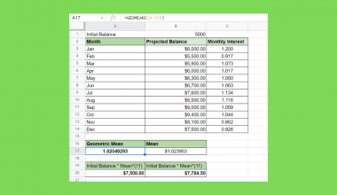
As one of the organizers of an annual quiz bee competition, you were given the task of creating a spreadsheet that will handle all the computations needed. It should be able to calculate the total points a contestant earns per round and the total score for the whole competition. It should also be able to quickly determine the rankings of the contestants based on the scores.

There are 3 rounds in the competition: easy, average, and difficult. A correct answer in each round corresponds to 5, 10, and 15 points, respectively. Data inputs should only be placing a number 1 to a corresponding cell if the contestant obtained the correct answer for that question. You draft up an example scenario and obtained the following:

You have successfully set up the spreadsheet such that the subtotal score per round and total points per contestant will be automatically computed. Now, the only thing left to do is to find a way to rank these scores automatically. This should allow you to determine the winners almost instantaneously without rearranging the dataset from highest to lowest total scores. How should you go about this problem?

Luckily, Google Sheets has a function that can easily solve this problem: the RANK function. It will return the rank of a specific value when the dataset is sorted in ascending or descending order.

Now, let’s get to know more about the RANK function in Google Sheets!

The Anatomy of the RANK Function

So the syntax (the way we write) the RANK function is as follows:

=RANK(value, data, [is_ascending])

Let’s dissect this thing and understand what each of these terms means:

= the equal sign is just how we start any function in Google Sheets.
RANK() this is our RANK function. It returns the rank of a specific value in a dataset. Rankings may be based on ascending or descending order.
value is the value whose rank will be determined. This value may be specified in the formula or it may be a cell reference.
data is the array or range that contains the dataset from where the rank of value will be obtained from. If data does not contain the value in any cell or element, the RANK function will return the #N/A error.
is_ascending determines how values in data will be arranged. The square brackets ‘[]’ indicate that this is an optional parameter. By default, its value is 0 when not specified – indicating data to be arranged in descending order. If a value of 1 is used, data will be arranged in ascending order. This means that the least value will have a rank of 1.

A Real Example of Using the RANK Function

Take a look at the example below to see how RANK functions are used in Google Sheets.

As you can see, the RANK function ranks the highest value in the dataset as 1 when the is_ascending parameter is not specified. If you want the lowest value to be ranked first, then this parameter should be specified as 1. Notice also how equal values in the dataset (the number 9 in cells A3 and A10) are ranked the same, taking the top rank of the entries.

You may make a copy of the spreadsheet using the link I have attached below:

Make a copy of example spreadsheet

How to Use the RANK Function in Google Sheets

Now, let’s finally use the RANK function to solve the example showed earlier.

Simply click on any cell to make it the active cell. For this guide, I will be selecting U3 where I want to show my result.

Next, simply type the equal sign ‘=’ to begin the function and then followed by the name of the function which is our ‘rank’ (or ’RANK’, whichever works). You should find that as you are typing, an auto-suggest box appears with the names of the functions that contain the text that you have typed.

The one we want is the RANK function so make sure to click on the RANK function. Alternatively, you may select the function by pressing the arrow down keys then pressing Enter or Tab to use the function (the currently selected function will be highlighted in grey and have a brief description below).

Upon selecting a function, a large text box appears that gives details about the function, and how to use the function. In some instances, a blue question mark will appear on the left side of the cell. If you want this text box to appear, simply click this question mark to show the large text box. Clicking on the arrow at the top right-hand corner will minimize the box while clicking on the x mark close the text box and the blue question mark will appear.

Now, we need to specify what the value to be ranked should be. For this example, I will first determine the rank of contestant 1. Select cell T3 and insert a comma ‘,’ to indicate that we would now like to input the data parameter.

To specify the data parameter, select the array containing the dataset to be considered. These are the values in cells T3:T12. Simply select this range and convert it to an absolute cell reference by pressing F4 on your keyboard once. This allows you to copy the formula down while keeping the same set of values for the data parameter.

Since we want the highest value to be ranked as the highest, let’s just leave the is_ascending parameter blank. Press Enter to finish the formula. To complete the table, simply copy the formula to the other rows.

The RANK function could also be used in conjunction with other functions like the ARRAYFORMULA function to make this process even faster and easier.

Using this additional function allows you to only edit the formula in one cell and the remaining cells will be automatically filled up. This also allows you more flexibility to add more values to the table and the ranks will automatically be updated. Feel free to follow the link provided to learn more about this function.

Another useful function is the IFNA function. This is a more specified version of the IFERROR function that allows you to specify a value when a formula returns the #N/A error. We already know that the RANK function returns the #N/A error when the value specified is not a part of the dataset considered. Therefore, any of the two functions can be used.

When you apply these two functions along with the RANK function for the example earlier, you should end up with the following table:

As you can see, you only need to input the formula for one cell and the remaining values will automatically be filled. Even though we have selected the entire T column as a part of the data set, an error prompt did not show because of the IFNA function.

That’s pretty much it. You can now use RANK functions in Google Sheets together with the other numerous Google Sheets formulas to create even more powerful formulas that can make your life much easier.