The TBILLEQ function in Google Sheets is useful when you need to calculate the equivalent annualized rate of return of a US Treasury Bill based on a provided discount rate.
A Treasury Bill or T-Bill is a short-term government security that matures in a year or less. The equivalent annualized rate of return is the actual interest rate of the bill after accounting for compounding.
The rules for using the TBILLEQ function in Google Sheets are as follows:
- The function requires the settlement date, maturity date, and discount rate of the bill at the time of purchase.
- The
TBILLEQfunction returns the equivalent annualized rate of return of the T-Bill.
Let’s take a look at a brief example of a situation where we might want to use the TBILLEQ function in Google Sheets!
In this example, we’ll be purchasing a Treasury Bill security. The settlement date of the security, or the date when the security is delivered to us, is on January 1st, 2021. The bill reaches its maturity date six months later on July 2nd, 2021. Given that the security has a discount rate of 2.5%, what is the equivalent annualized rate of return of the indicated bill?
With the TBILLEQ function, it becomes quite easy to calculate the annualized rate of return. Now we know one example of when we can use the TBILLEQ function. Let’s now dive into how to use this function and work on an actual sample spreadsheet.
The Anatomy of the TBILLEQ Function
So the syntax (the way we write) of the TBILLEQ function is as follows:
=TBILLEQ(settlement, maturity, discount)
Let’s dissect this thing and understand what each of these terms means:
- = the equal sign is how we start any function in Google Sheets.
- TBILLEQ() is our
TBILLEQfunction. It computes the equivalent annualized rate of return of a US Treasury Bill based on a given discount rate - settlement refers to the security’s settlement date.
- maturity refers to the security’s end date or maturity date, when the security can be redeemed at face value.
- discount refers to the discount rate of the treasury bill.
A Real Example of Using TBILLEQ Function
Let’s look at an example of the TBILLEQ function being used in a Google Sheets spreadsheet.
As seen in the worksheet below, we set up a calculator for the Annual Equivalent Rate of Return of a US Treasury Bill. We have our values for the settlement date, maturity date, and discount rate.
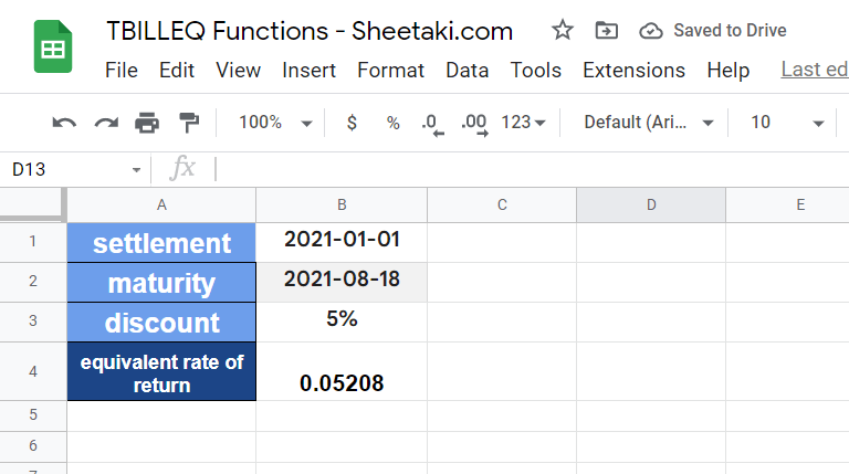
With these given values, we can now compute the equivalent rate of return of our bill.
Given the current values, the annual equivalent rate of return of our Treasury Bill is 0.05208. This means that the return on the investment is 5%, accounting for compounding.
Feel free to copy the spreadsheet above using the link attached below.
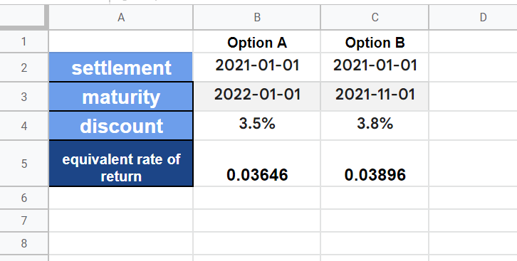
As another example, we can create a worksheet that compares the rate of return of different treasury bill options. In the table below, we use the TBILLEQ formula in Google Sheets to calculate the rate of return of both options.
Now that we’ve explored a sample usage of the TBILLEQ function in Google Sheets, let’s begin writing it ourselves!
How to Use TBILLEQ Function in Google Sheets
- To set up our Treasury Bill Yield calculator, we should set up the arguments needed.

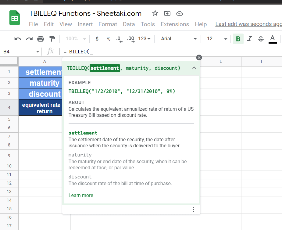
- In cell B4, we can start typing out our function. We just simply input the equal sign ‘=‘ to begin the formula, followed by ‘TBILLPRICE(‘.
- As seen below, a tooltip box appears with info on the
TBILLEQfunction. We can click on the arrow on the top-right-hand corner of the box to minimize it if necessary.
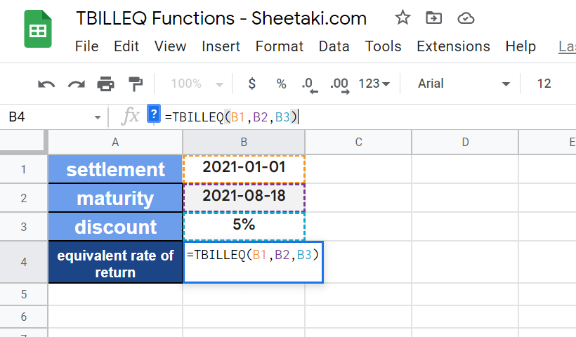
- Lastly, we should reference cells containing the values needed to compute the rate, as seen below. Afterward, simply hit Enter on your keyboard to let the function evaluate.
Frequently Asked Questions (FAQ)
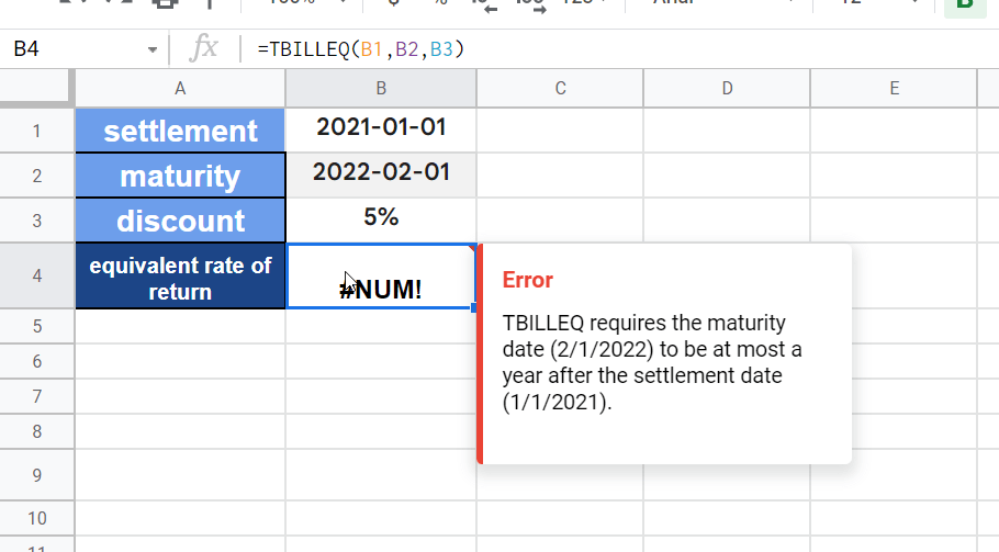
- Why does my formula return a #NUM! error?
TheTBILLEQfunction returns a #NUM! error if the time between the settlement date and the maturity date is over one year. This is because US Treasury Bills have a maturity of a year or less. In the example below, the maturity price is over a year after the settlement date, causing the formula to return an error.
- Why does my formula return a #VALUE! error?
If you receive a #VALUE! error, you can try to verify if either the settlement date or the maturity date is invalid. To prevent errors from invalid dates, we can use theDATEformula or use data validation.
Alternatively, there may be a non-numeric value in one of your arguments that might be causing the error.
Now we’ve shown you everything you need to use the TBILLEQ function in Google Sheets. This guide shows how easy it is to compute the annual rate of return of a given US Treasury bill.
You can now use the TBILLEQ functions in Google Sheets together with the various other Google Sheets formulas available to create great worksheets that work for you. Stay notified of new Google Sheets guides like this by subscribing to our newsletter!