


This guide will discuss how to perform data binning using three simple methods in Excel.
Excel is a popular tool used by different people for various purposes and situations. Since it has several built-in functions and tools, we can easily perform difficult and time-consuming tasks such as data analysis and data summarizing.
When we have a large quantity of data, it is better to summarize them to analyze and understand the data easily. For example, data binning is a common and easy way to summarize large quantities of data, especially continuous data.
Data binning is placing numeric data into groups called bins to easily determine the distribution of values in a given data set. However, data binning can be a time-consuming process since it deals with a large quantity of continuous numeric data.
Since the basic idea of data binning is to place the numeric data into groups called bins, we can simply create bin ranges in Excel using three simple methods. Moreover, histograms utilize bin ranges in their X-axis, so we can simply create a histogram to perform data binning.
Firstly, we can simply use the built-in charts available in Excel to create a histogram. Secondly, we can also utilize the data analysis tool in Excel to make a histogram. Lastly, we can use the FREQUENCY function to create the bin ranges and then make a graph using the results.
Let’s take a sample scenario wherein we need to perform data binning in Excel.
Suppose you are a teacher who wants to understand the students’ performances in class based on their test scores. So you performed data binning to group the students’ grades and determine the number of students lagging behind.
To do this, you simply utilized the built-in charts in Excel and created a histogram with your data set. And this way, you can easily check the bin ranges on the X-axis of the histogram.
Before we dive into the methods of performing data binning in Excel, let’s first learn the syntax of the FREQUENCY function.
The Anatomy of the FREQUENCY Function
The syntax or the way we write the FREQUENCY function is as follows:
=FREQUENCY(data_array, bins_array)
Let’s take apart this formula and understand what each term means:
- = the equal sign is how we activate any function in Excel.
- FREQUENCY() is our
FREQUENCYfunction. And this function is used to calculate how often values occur within a given range of values. Then, the function will return a vertical array of numbers having one more element than the bins_array argument. - data_array is a required argument. So this argument refers to an array or cell reference to a set of values for which we want to count the frequencies. Furthermore, the blanks and text values are ignored in the count.
- bins_array is also a required argument. And this refers to an array or cell reference to intervals into which we want to group the values counted in the data_array argument.
Great! Now we can move on and discuss the three simple methods we can use to perform data binning in Excel.
How to Perform Data Binning in Excel Using Built-in Charts
Firstly, we can easily create a data bin in Excel by inserting a histogram. So a histogram is a bar chart that displays frequency counts in bin ranges. Furthermore, Excel already has a built-in histogram chart available. So we can simply insert a histogram using the values in our data set.
Then, we can identify the bin ranges by looking at the X-axis of the histogram and determine the frequency of each bin range by the bar.
To apply this method to your work, we can simply follow the steps below.
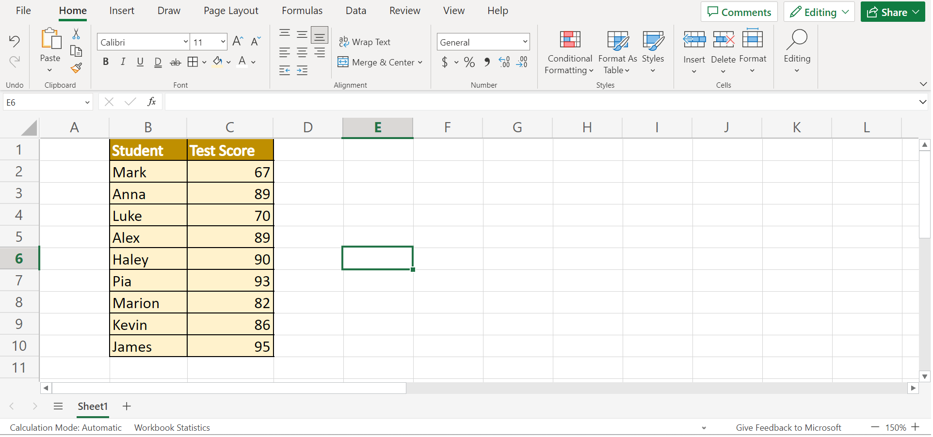
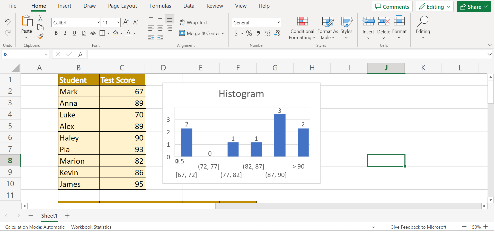
1. Firstly, we prepare our data set. In this case, we have listed 9 students alongside their test scores.
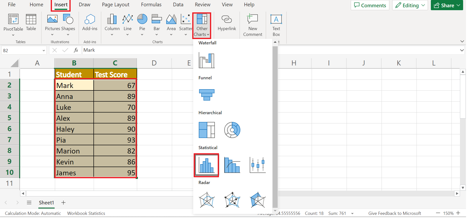
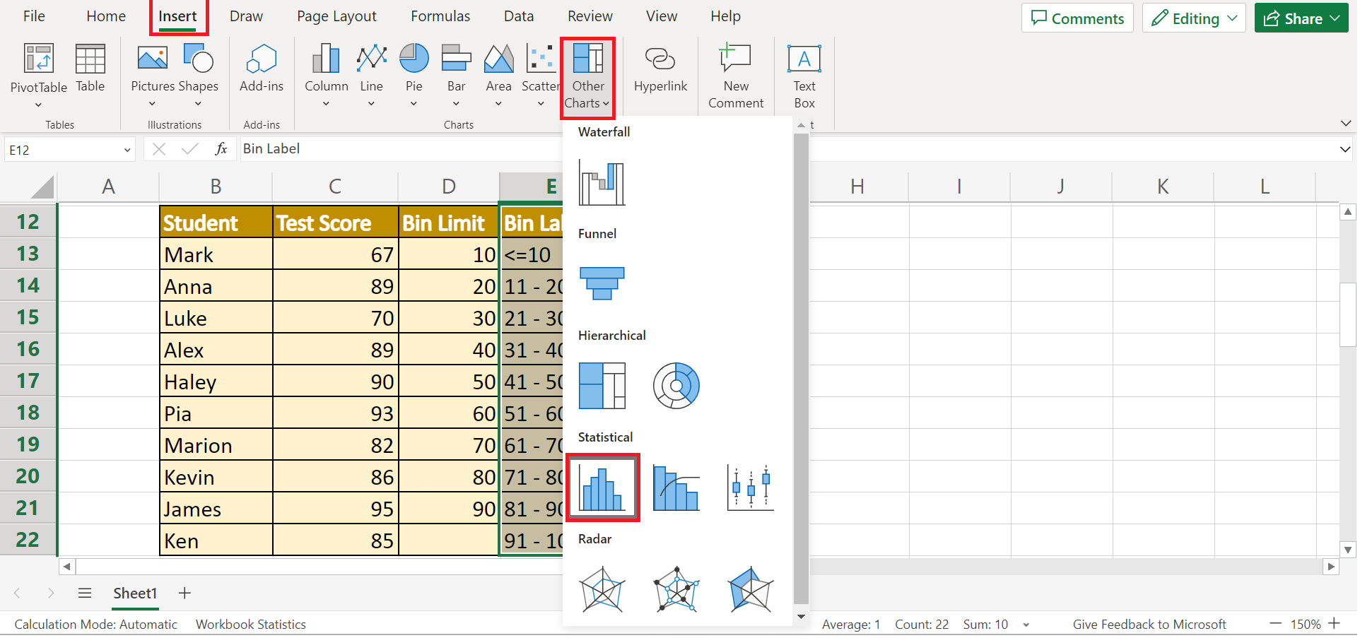
2. Secondly, we will select our entire data set and go to the Insert tab. Next, we will select the Other Charts. Then, we will choose the Histogram icon in the dropdown menu.
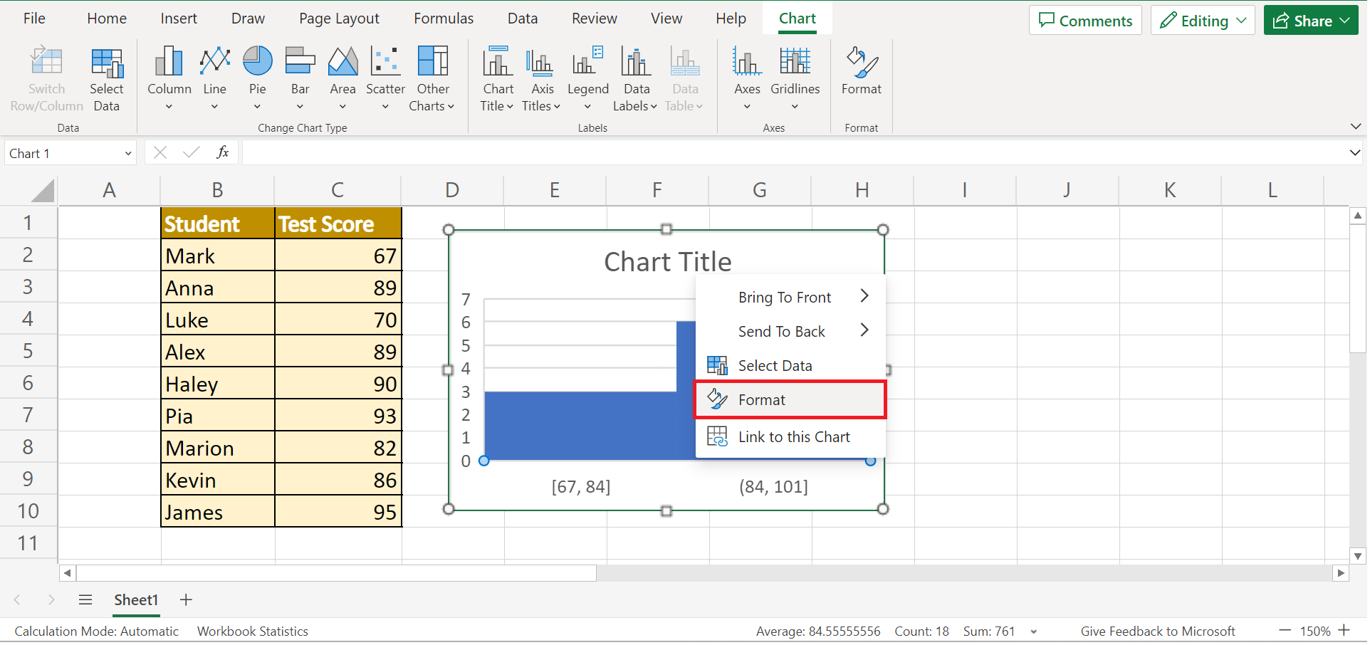
3. Thirdly, we will format our bin ranges. To do this, we will right-click the chart and select Format.
4. Next, we will change the Bin width to what we need. In this case, we will input “5” as our Bin width. We will also select Overflow bin and Underflow bin to express the range on which the histogram will plot.
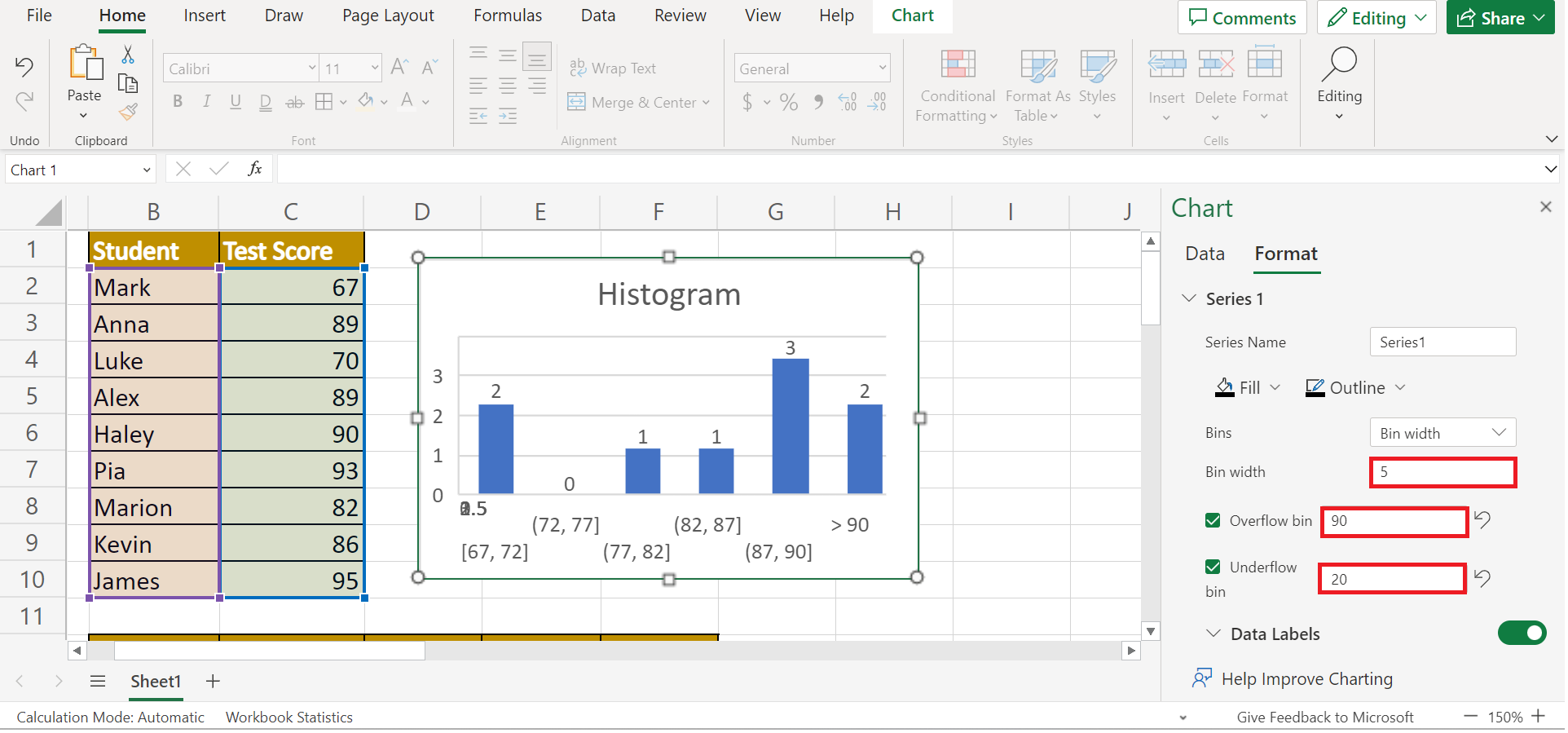
5. Furthermore, we can edit the histogram and add labels. To do this, we can simply turn on Data Labels.
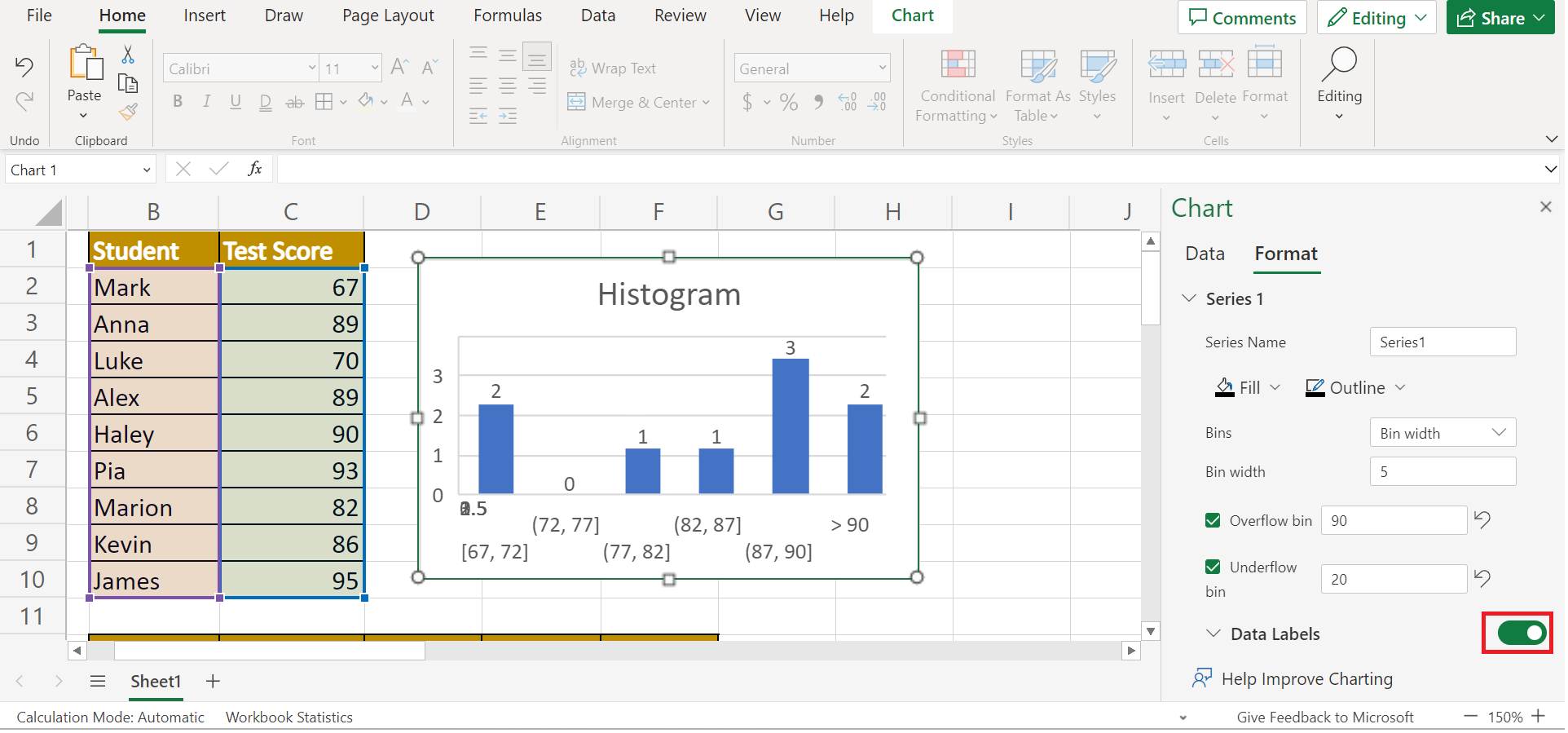
6. And tada! We have successfully performed data binning in Excel.
How to Perform Data Binning in Excel Using Data Analysis
Secondly, we can utilize the free analysis toolpak in Excel to perform data binning. In this method, we would need to first create our bins. Then, we will use the data analysis feature to create a histogram. And this will allow us to place our values into their corresponding bins.
To use this method in your work, we can simply follow the steps below.
1. Firstly, we need to install the Analysis Toolpak in Excel. So we will go to the File tab and select More. then, we will click on Options.
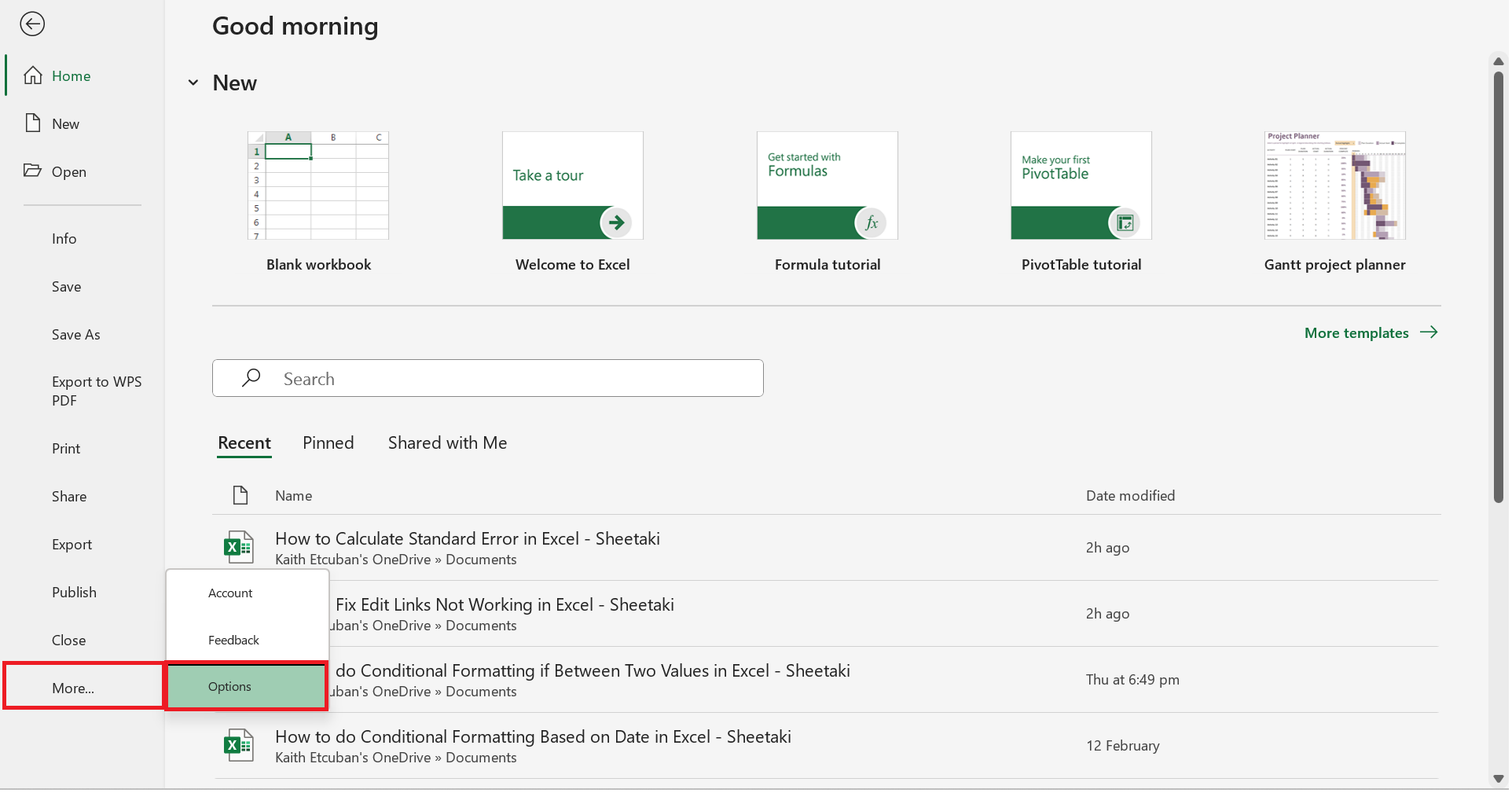
If you already have the Data Analysis feature in your ribbon, you can skip these steps and proceed to step 4.
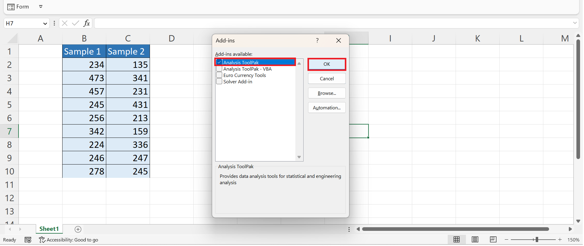
2. Secondly, we will click Add-ins and choose Analysis ToolPak from the available list. Lastly, we will click Go.
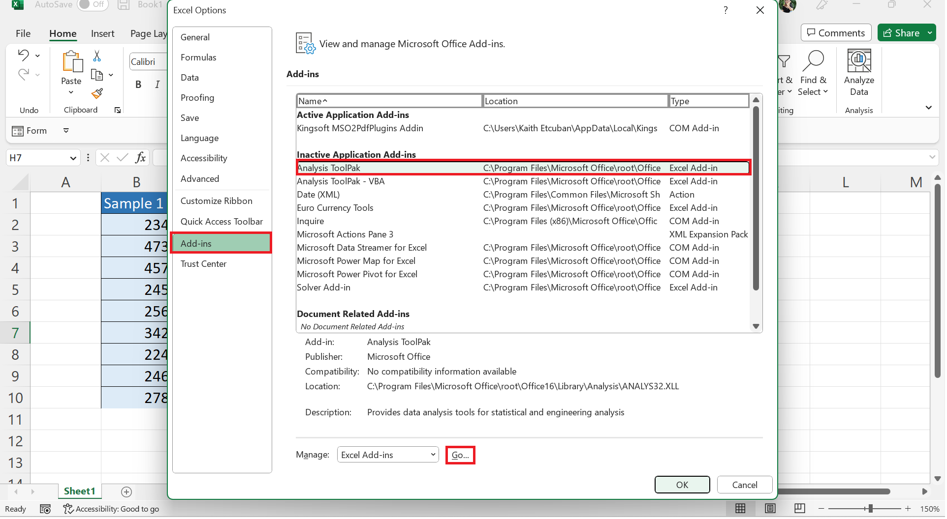
3. Thirdly, we will choose Analysis ToolPak and click OK.
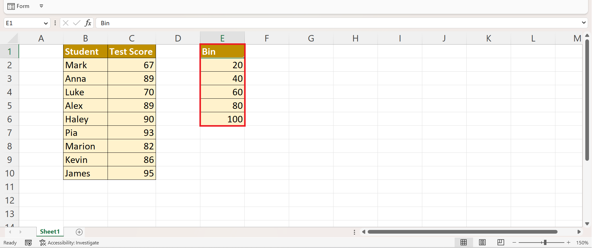
4. Next, we need to define the largest value for each bin. In this case, we want each bin to have a range of 20.
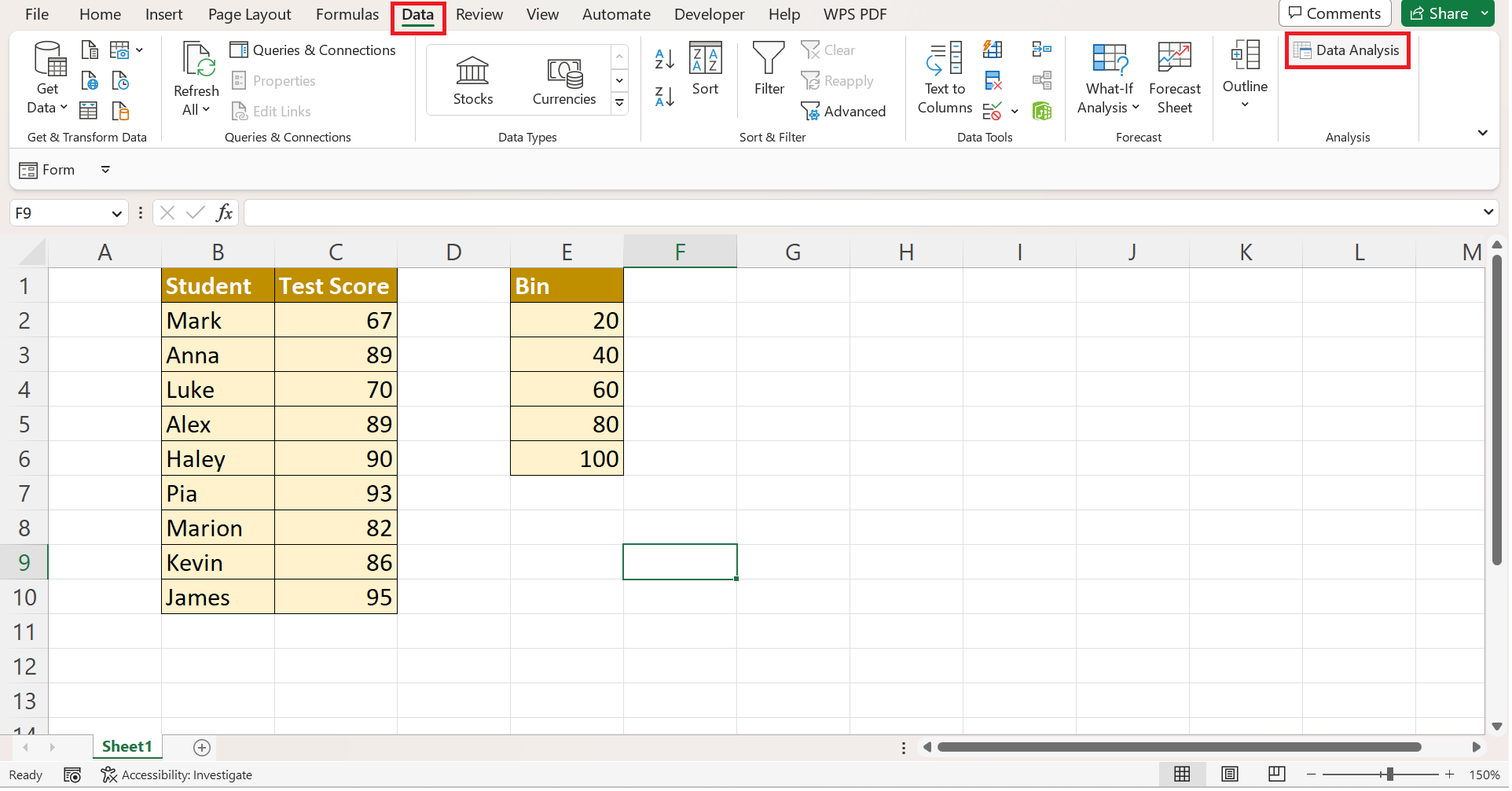
5. Then, we will go to the Data tab and select Data Analysis.
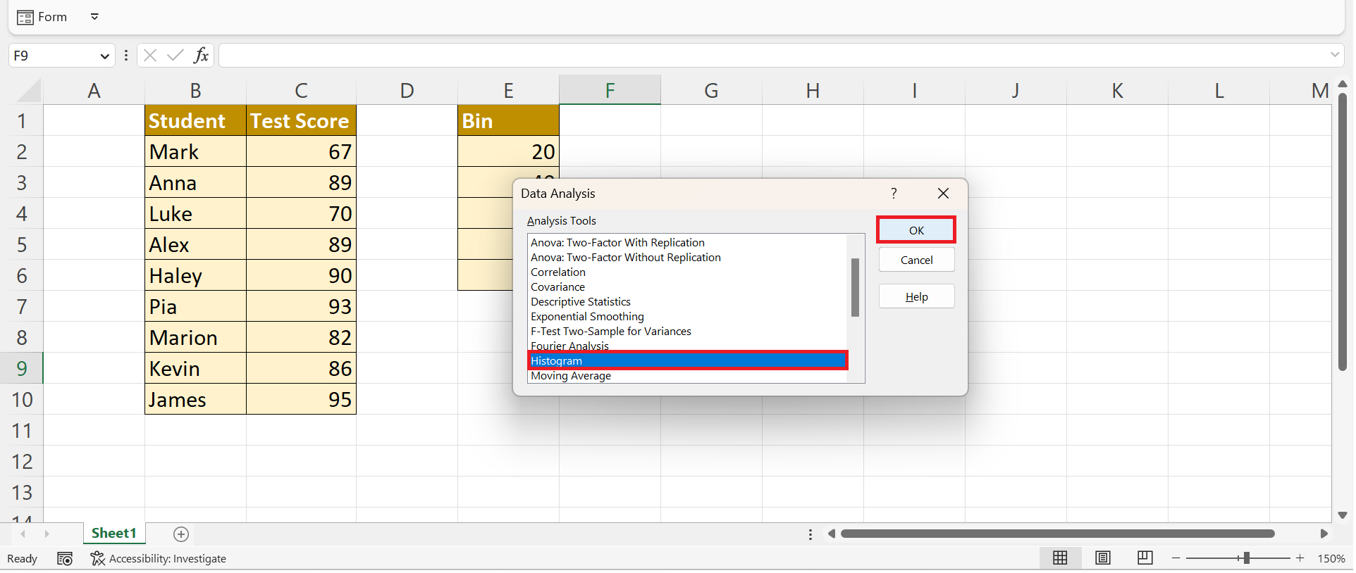
6. Afterward, we will select Histogram and click OK.
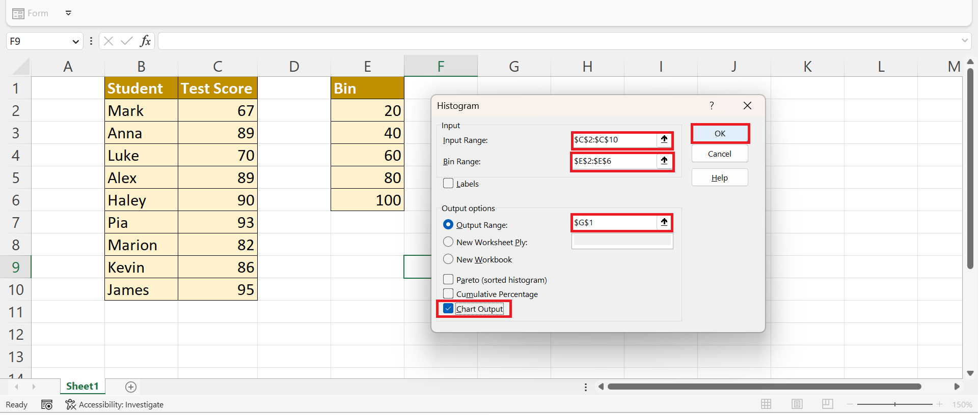
7. In the window, we will select our bin ranges as our Input Range and select an empty cell for our Output Range. Next, we will check the box for Chart Output. Lastly, we will click OK.
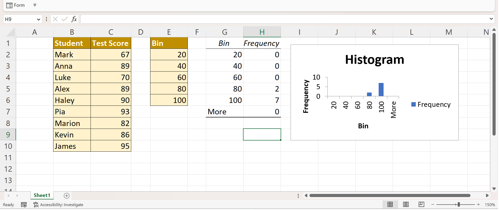
8. And tada! It will automatically create a histogram that displays the number of values that fit each bin.
How to Perform Data Binning in Excel Using FREQUENCY
Lastly, we can perform data binning in Excel using the FREQUENCY function. So the FREQUENCY function calculates how often values appear within a given range.
To apply this method, we can simply follow the steps below.
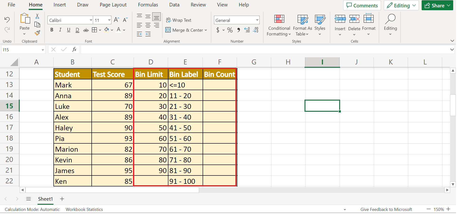
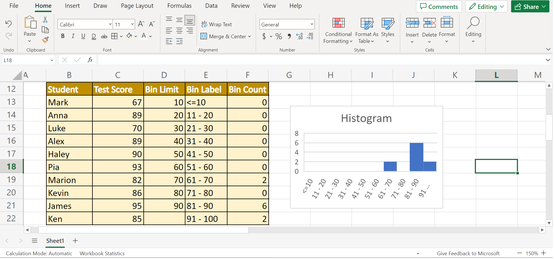
1. Firstly, we must create our table, including the Bin Limit, Bin Label, and Bin Counts. In the Bin Limit, we will input the largest value possible in the range. In Bin Label, we will input the range.
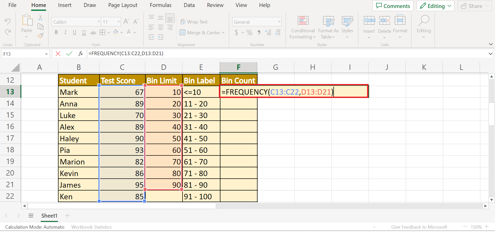
2. Secondly, we will place the formula “=FREQUENCY(C13:C22,D13:D21)” in the first cell of our Bin Counts column. Lastly, we will press the Enter key to return the results.
3. Thirdly, we will select the Bin Label and Bin Counts columns. Next, we will go to the Insert tab. Then, we will select Other Charts and choose the Histogram icon.
4. And tada! We have successfully used the FREQUENCY function to perform data binning.
You can make your own copy of the spreadsheet above using the link attached below.
And that’s pretty much it! We have discussed how to perform data binning using three simple methods in Excel. Now you can choose and apply any of the methods to your work.
Are you interested in learning more about what Excel can do? You can now use the FREQUENCY function and the various other Microsoft Excel formulas available to create great worksheets that work for you. Make sure to subscribe to our newsletter to be the first to know about the latest guides and tutorials from us.


