How to Pick a Random Name from a Long List in Google Sheets

You can easily create a random draw winner selection tool to pick a random name from a long list in Google Sheets.

It is useful if you have a list of names in one column and want to draw between them.

Say you have a competition for your website, school, or workplace, and you need to pick a random winner from a long list.

So how do we do that?

I will show you a solution using the combination of three Google Sheets functions:

• COUNTA to count the number of participants in the draw,
• RANDBETWEEN to pick a random number between 1 and the total number of participants,
• INDEX finally to match the randomly selected number with the corresponding name in the list.

Let’s dive right into real examples to see how to pick a random name from a long list in Google Sheets.

The Anatomy of the RANDBETWEEN and INDEX Functions

The Anatomy of the RANDBETWEEN Function

The RANDBETWEEN function is a random number generating function. The syntax of the RANDBETWEEN function is as follows:

=RANDBETWEEN(low, high)

Let’s see what each part of this means:

• = the equal sign is just how we start any function in Google Sheets.
• RANDBETWEEN is our function. We will have to add the arguments into it to work.
• low means the low end (the smallest number) of the random range.
• high is the high end (the biggest number) of the random range.

For example, we need a random number between 1 and the total number of names to pick a random winner.

We can write the exact number of participants if it is always the same. For instance, if there are always 12 names in our list, we can write this function in the following way:

=RANDBETWEEN(1, 12)

However, it is highly possible that you either don’t know the exact number of names or it changes.

This is why the COUNTA function is useful. It counts the number of cells in a selected range. Therefore, we use it with a column reference that contains all the names we want to include in the calculation.

If the list of the names is in column A starting from A2, then you can write the following formula:

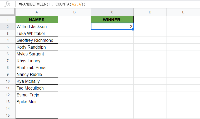
=RANDBETWEEN(1, COUNTA(A2:A))

This function returns a random number which we can use as the index of the selected winner.

Great, we know how to pick a random winner! But we need to see his name as well. So we need to identify the randomly picked number and show the corresponding name of the list.

The Anatomy of the INDEX Function

The INDEX function is useful to return the content of a cell, specified by row and column offset.

The syntax of the INDEX function is as follows:

=INDEX(reference, row, column)

Let’s dissect this thing and see what each part of this means:

• = the equal sign is just how we start any function in Google Sheets.
• INDEX is our function. We will have to add the arguments into it to work.
• reference means the range of cells where the values are located.
• row is an optional argument. It means the number of offset row(s) from the range.
• column is also an optional argument, it means the number of offset column from the range.

We want to pick a random number from a long list. Hence, we will need to use the list of the names as reference, and then the randomly selected number as row.

This way, we can match the randomly picked number with its corresponding name from the list.

A Real Example of Using RANDBETWEEN and INDEX Functions

Let’s see how we can use all this to pick a random name from a long list in Google Sheets.

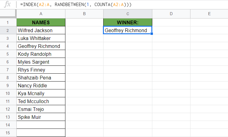
As you can see in the image above, the combination of the three functions shows a randomly picked name from the list. The function is as follows:

=INDEX(A2:A, RANDBETWEEN(1, COUNTA(A2:A)))

Here’s what this example does:

• We have actively selected the cell (or box) under C2, where we want to put our randomly picked name. As you can see, we use the INDEX function wrapping the RANDBETWEEN function wrapping the COUNTA function.
• We need to give two arguments to the INDEX function. First, we need to add the range of cells where the names are written. We select the cells from A2 until the end of column A as our first argument in the INDEX function.
• And then, we need the row variable, which is the randomly picked number. We write a RANDBETWEEN function here to select a random number between 1 and the total number of names.
• The RANDBETWEEN function has two arguments, low and high. The first argument (low) means the smallest index in the list, which is 1.
• After that, the second argument (high) is the largest number we would like to include in our random number picker, so it is the total number of names. We use the COUNTA function to calculate how many names are written in column A, starting from cell A2, so the argument is A2:A.
• As you can see, the value ‘Geoffrey Richmond‘ was inserted into our selected C2 because this is the random name the function picked for us.

Try it out by yourself. You may make a copy of the spreadsheet using the link I have attached below and try it for yourself:

How to Pick a Random Name from a Long List in Google Sheets

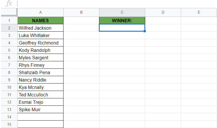
1. Simply click on any cell to make it the active cell. For this guide, I will be selecting C2, where I want to show my result.

2. Firstly, start by writing the RANDBETWEEN function to pick a random number between 1 and the total number of names. Simply type the equal sign ‘=‘ to begin the function and then followed by the name of the function which is our ‘randbetween‘ (or ‘RANDBETWEEN‘, whichever works).

3. Great! Now you should find that the auto-suggest box will pop-up with the names of the functions. The one we want is our RANDBETWEEN function. So make sure to click on the right one!

4. Now what you need to do is select the low and high values that you want to use the RANDBETWEEN function with. You need 1 as the low value, so you need to write it as the first argument of the function.

5. After that, you need to calculate the total number of names, which will be the second argument. You need to use the COUNTA function. After the first argument, type a comma and start typing the name of the function which is ‘COUNTA’. Make sure to select the right one! Type a bracket after the COUNTA function name (Google Sheets will auto-fill it most of the time).

6. The argument we need in the COUNTA function is the whole range of cells containing the names. Therefore, you need to include all the cells where it is possible to later have new additional names. So, in my example, I will be selecting the whole column A starting from cell A2. I need to write it as A2:A.

7. Great! Close the brackets on both of the functions. So far, you created the random number picker that chooses a number between 1 and the total number of names.

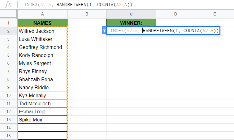
8. Now, you need to use the INDEX function to show the name of the picked winner. The INDEX function has to wrap the whole random number picker, so you need to type the name of the function at the beginning of the formula.

9. The INDEX formula needs two arguments and one of them (the second one, row) is the already written RANDBETWEEN formula. So you only need to add the first argument that is reference. You need the range with the names here as reference argument, which is the range A2:A in my example. Let’s type this before the RANDBETWEEN formula.

10. Finally, just close all the functions with the closing brackets ‘)‘ then hit your Enter key. You’ll find a randomly picked name in the cell C2.

That’s it, good job! You can now pick a random name from a long list together with the other numerous Google Sheets formulas to create even more powerful formulas that can make your life much easier. 🙂

Get emails from us about Google Sheets.

Our goal this year is to create lots of rich, bite-sized tutorials for Google Sheets users like you. If you liked this one, you'll love what we are working on! Readers receive ✨ early access ✨ to new content.

Subscribe