How to Generate Random Numbers in Google Sheets

Learning how to generate random numbers in Google Sheets is useful to create a unique number that does not carry any recognizable pattern.

Generally, random number generators are applied to gambling, statistical sampling, computer simulation to produce completely randomized designs to have unpredictable results. 

For example, students want to generate random numbers to select samples for their research quickly. They can use Google Sheets to create randomized numbers by applying these two functions:

1. RANDBETWEEN function
2. RAND function

The Anatomy of the RANDBETWEEN Function

The way we write the RANDBETWEEN function is:

=RANDBETWEEN(low, high)

Let us help you understand the context of the function:

• The equal sign =  is how we start any function in Google Sheets.
• RANDBETWEEN() is our function. To make the function work correctly, we need to add two attributes, namely the low and high.
• The low is the lower integer of the random range.
• The high is the higher integer of the random range.

How the RANDBETWEEN function works lets you generate a random integer between the given range. Hence, you will need to specify a lower and upper limit to set the range.

You should take note that the RANDBETWEEN function only returns in integers. Meaning the numbers generated are whole numbers.

Let us use a real-life example to demonstrate how to use the RANDBETWEEN function.

A Real Example of Using RANDBETWEEN Function

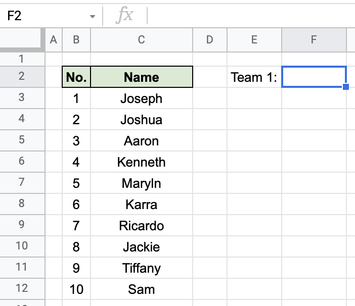
In this example, we would like to generate a set of randomized numbers to group all ten participants into two separate groups.

We are going to use the RANDBETWEEN function to generate five random numbers to form the first group. The remaining numbers would be group two.

Let us go through how to generate these five random numbers step-by-step!

How to Use the RANDBETWEEN Function in Google Sheets

1. Simply click on the cell that you want to write down your function at. In this example, it will be F2.

2. Begin your function with an equal sign =, followed by the name of the function, RANDBETWEEN, then an open parenthesis (.

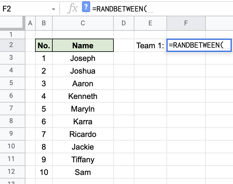
3. We will first type in the lowest integer which is ‘1’, followed by the highest integer, which is ‘10’. Then we will copy the same formula to the four cells below to generate four more random numbers.

By generating these five numbers, we can group one team of participants according to those numbers and the remaining into another team.

However, there are some shortfalls in using the RANDBETWEEN function to generate random numbers. Let us explain why:

1. The RANDBETWEEN function can only generate whole numbers and is unable to generate decimal numbers. 
2. The RANDBETWEEN function only works well when there is a large range and is used to generate a small range of random numbers.

For example, if you would like to generate unique random numbers with a small range, the RANDBETWEEN function would generate repeated random numbers. Hence, it may not be a suitable function. 

Another great function that can generate random numbers is the RAND function. This function can generate random numbers in decimal form.

The Anatomy of the RAND Function

The way we write the RAND function is:

=RAND( )

Let us help you understand the context of the function:

• The equal sign =  is how we start any function in Google Sheets.
• RAND() is our function. 

The RAND function is also a simple function to use. As you can see, it does not need any input to make the function work. 

How to Use the RAND Function in Google Sheets

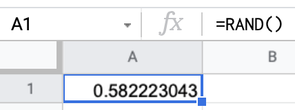
Without inputting any parameters into the function, it would generate a random number between zero and one. The numbers randomly generated would be more than or equal to zero and lesser than one.

Example 1

We can also set a lower and upper limit to generate a random decimal number by tweaking the formula.

For example, if we want to generate a random number between one and five.

Here is a visualization of how the formula works:

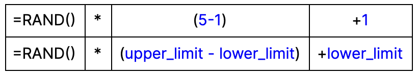
By doing so, we can generate a random decimal number in any range of numbers.

Example 2

The RAND function can be used with the ROUND function to reduce the decimal numbers to your preference. 

The ROUND function can help to round down or round up to help provide a more manageable number. You can also learn more about this function through our written tutorial and examples on the ROUND function. 

For example, you want the randomly generated numbers to only have two decimals.

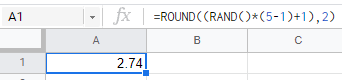
Here is a visualization of how the formula works:

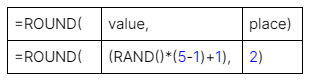
In this formula, the RAND function has become the value. By inputting ‘2’ as the integer in the ROUND function signifies the function to only return a random number in two decimals.

Example 3

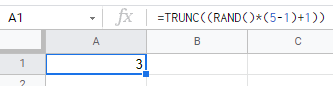
Another function that can be used together with the RAND function is the TRUNC function. Instead of rounding up or down like the ROUND function, the TRUNC function helps you to make the randomly generated number whole. 

The TRUNC function works with two arguments:

=TRUNC(number,[num_digits])

Hence, the RAND formula has now become the number within the TRUNC formula. 

The num_digit is an optional argument. If there are no numbers inputted for this argument, it will default to zero. If you input a number for this argument, it will help specify the precision for the number to truncate to.

The TRUNC function also works similarly to the ROUND function. If we specify a number for the num_digit argument, it will signify how many decimals the formula would return.

For example, if you want the formula to return four decimals.

All you need to do is to add four as the num_digit instead of leaving it blank like the previous example. 

You may make a copy of the spreadsheet using the link I have attached below. 

Refresh Rate of the RANDBETWEEN and RAND Functions

By now you must have realized the constantly changing numbers randomly generated by these two functions. 

This is because these are volatile functions that constantly refresh once changes are made to the spreadsheet.

One way to slow down the refresh rate of these functions is to manually change the specifications of the spreadsheet.

1. First, press File, then select Spreadsheet settings.

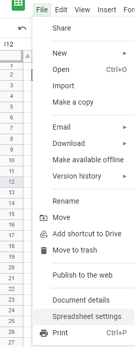
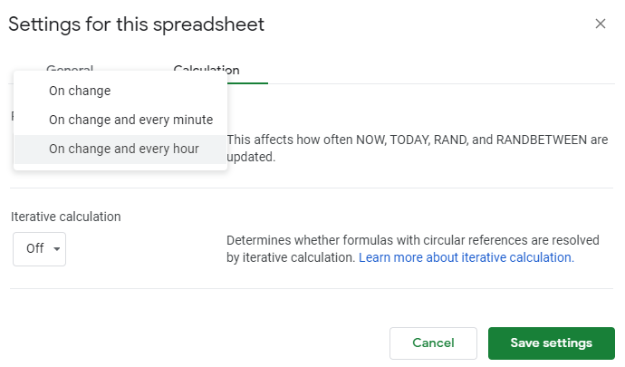
2. Then, on the top bar, select Calculation. 

3. Select On change and every hour for the recalculation settings. Finally, press Save settings, and you are done!

There you go! Two different ways to generate random numbers to your preference and specifications. 

Don’t forget to check out other cool functions in Google Sheets to enhance and simplify work for your everyday use!

Get emails from us about Google Sheets.

Our goal this year is to create lots of rich, bite-sized tutorials for Google Sheets users like you. If you liked this one, you'll love what we are working on! Readers receive ✨ early access ✨ to new content.

Subscribe