How to Round Significant Figures in Excel

This guide will discuss how to round significant figures in Excel using the ROUND function in two simple and easy methods. 

The rules for using the ROUND function in Excel are the following:

• The ROUND function can support rounding to the right and left of the decimal point.
• When the last significant digit of the selected value is 5 or greater than 5, the function will round up.
• When the last significant digit of the selected value is less than 5, the function will round down.
• If the inputted value for num_digits is greater than zero, the function will round on the right side of the decimal point. So we input zero in num_digits when we want to round to the nearest integer.
• When the num_digits argument has a value less than or equal to zero, the function will round on the left side of the decimal point. 

Excel is an excellent tool to use when performing complicated and lengthy calculations. And it contains several built-in functions we can use and manipulate for different purposes.

For example, we want to round our values to significant figures. So significant figures refer to several digits that carry or apply meaningful contributions to the measurements or values of the data set as a whole. 

In this case, we can use the ROUND function in Excel to create two formulas that will easily round our values to their significant figures. Furthermore, we will combine other built-in functions in Excel with the ROUND function to create these two formulas. 

Let’s take a sample scenario wherein we need to round significant figures in Excel.

Suppose you have a list of numeric values. Let’s say you have performed long calculations. And now, you want to round the values to the significant figures as the final result. 

To make this task easier, you applied the ROUND function together with different functions, such as the INT function, LOG10 function, and ABS function, to create a formula that will round significant figures. 

Before we move on to a real example of rounding significant figures in Excel, let’s first learn about the functions we will use to perform this task.

The Anatomy of the ROUND Function

The syntax or the way we write the ROUND function is as follows:

=ROUND(number, num_digits)

Let’s take apart this formula and understand what each term means:

• = the equal sign is how to start any function in Excel.
• ROUND() refers to our ROUND function. And this function is used to round a number to a specified number of digits. In other words, this function will round up or round down based on the last digits of the selected value.
• number is a required argument. So this refers to the number we select or input that we want to round up or round down.
• num_digits is another required argument. And it refers to the number of digits to which we want to round the selected value. Specifically, negative values round to the left of the decimal point, while zero rounds to the nearest integer. 

The Anatomy of the LOG10 Function

The syntax or the way we write the LOG10 function is as follows:

=LOG10(number)

Let’s take apart this formula and understand what each term means:

• = the equal sign is how we activate any function in Excel.
• LOG10() is our LOG10 function. And this function is used to return the base-10 logarithm of a selected or inputted number.
• number is the only required argument for this function. So this refers to the positive real number for which we want the base-10 logarithm. 

Great! Now we can move on to a real example of rounding significant figures in Excel.

A Real Example of Rounding Significant Figures in Excel

Let’s say we have a data set containing a list of numeric values. And we need to round the values to their significant figures as the final result. So our initial data set would look like this:

In this case, we have a list of the monthly sales in 8 digits. Since we want to round these values to specific significant figures, we can use two easy and simple methods.

Firstly, we can use a formula combining the ROUND function with the INT function, LOG10 function, and ABS function to round the values to their significant figures. So the formula will first return a value with a positive sign using the ABS function.

Then, the formula will return the base-10 logarithm result of the value we selected using the LOG10 function. Next, the INT function will retire the nearest lower integer value of the result. Afterward, the three functions will be used to give the number of significant figures to round. 

Lastly, the ROUND function will round the values depending on the results.  

Secondly, we can use another method to round significant figures in Excel. We will use the ROUND function with the INT and LOG10 functions to create a formula. So this method will allow you to easily change the number of significant figures to make a dynamic work. 

So the formula will use the LOG10 function to return the 10-based logarithmic result of the value we selected. Then, the INT function will return the nearest lower integer of the value from the LOG10 function. Afterward, we will convert the inputted value to a fraction. 

Next, the ROUND function in the formula will round the fraction number to the specific significant figure we have inputted. Lastly, we will multiply the rounded fraction based on the formula’s calculations. And this method will allow you to change the number of significant figures by simply changing the value. 

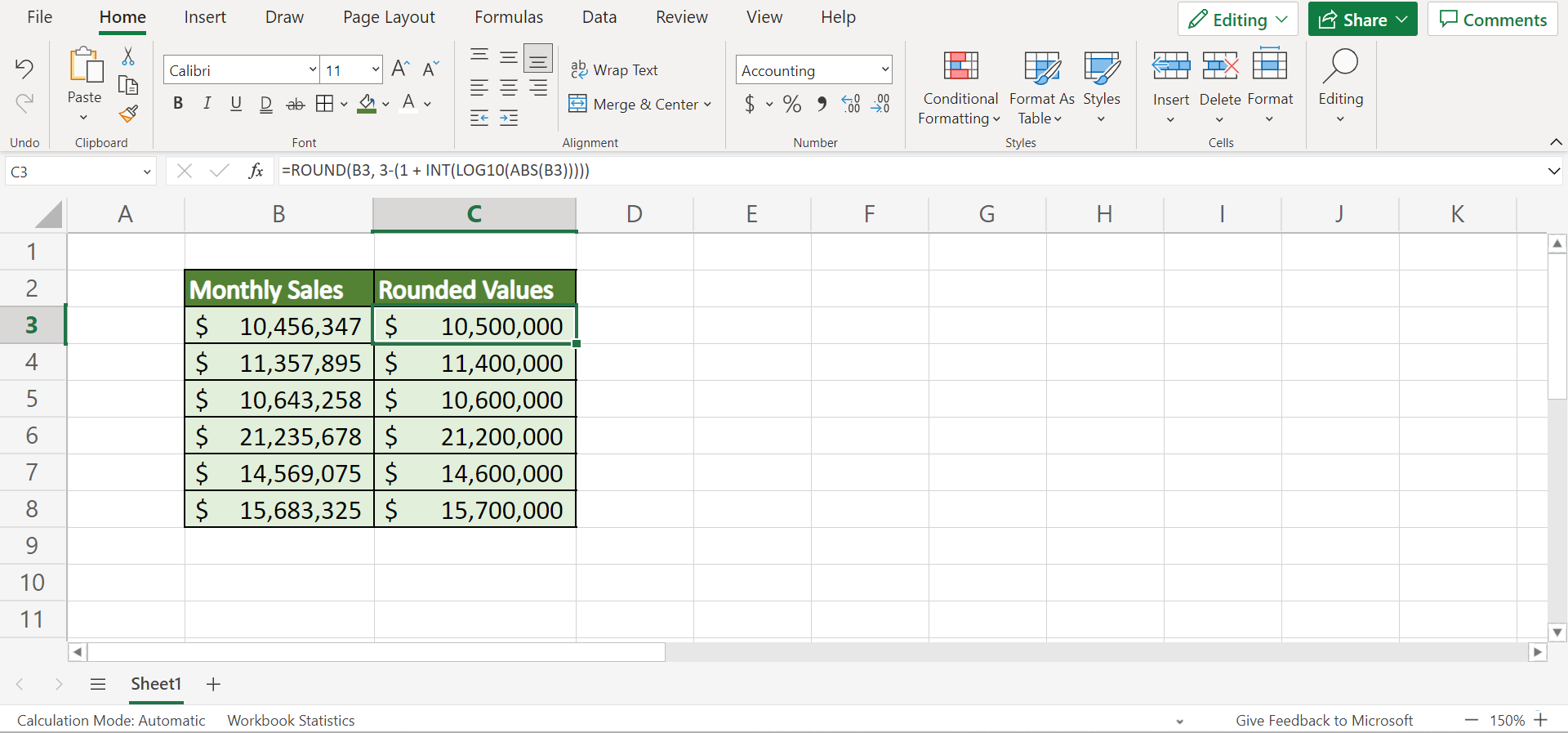
So our final data set would look like this:

You can make your own copy of the spreadsheet above using the link attached below. 

Amazing! Now let’s move on and dive into the steps of how to round significant figures in Excel.

How to Round Significant Figures in Excel

In this section, we will discuss the step-by-step process of how to round significant figures in Excel using two simple and easy methods. Additionally, each step has detailed instructions and pictures to help you through the process.

1. Firstly, we will create a new column wherein we will input the results. Then, we can use the first method to round significant figures. In this case, we can simply type in the formula “=ROUND(B3, 3-(1 + INT(LOG10(ABS(B3)))))”. Lastly, we will press the Enter key to return the result.

2. Secondly, we will drag down the Fill Handle tool to copy the formula to the other cells.

3. And tada! We have successfully rounded significant figures in Excel.

4. Now, let’s try another dynamic method that will allow us to change the number of significant figures whenever necessary. Firstly, we need to make a cell to indicate the significant figures.

5. Then, we will input the formula “=ROUND(B3/10^(INT(LOG10(B3)) + 1), $E$3)* 10^(INT(LOG10(B3))+1)”. Finally, we will press the Enter key to return the result.

6. Next, we will drag the Fill Handle tool down to copy and apply the formula to the other cells.

7. Now we can simply change the value in the significant figures whenever we want to round the values to different significant figures.

And that’s pretty much it! We have discussed how to round significant figures in Excel using two simple and easy methods. 

Are you interested in learning more about what Excel can do? You can now use the ROUND function and the various other Microsoft Excel formulas available to create great worksheets that work for you. Make sure to subscribe to our newsletter to be the first to know about the latest guides and tutorials from us.

Get emails from us about Google Sheets.

Our goal this year is to create lots of rich, bite-sized tutorials for Google Sheets users like you. If you liked this one, you'll love what we are working on! Readers receive ✨ early access ✨ to new content.

Subscribe