How to Hide All Error Values in Excel

We can use the IFERROR function and conditional formatting to hide all error values in a Microsoft Excel spreadsheet.

This technique will be useful for cleaning up a table that may be prone to errors.

Common Excel errors include the #DIV/0, #REF, and #VALUE errors. While these error outputs are incredibly useful for finding bugs in your spreadsheet, they may be distracting. This is especially the case with spreadsheets where errors are expected, such as a table with missing values.

For example, let’s say we have a table where a column is the quotient of two other values. If the divisor is zero, then our column will return a #DIV/0 error. While dividing by zero is considered an error in mathematics, a blank cell may be easier to read for users.

With this situation in mind, is it possible to hide error values from your worksheet?

Excel’s IFERROR function can help catch these errors when they happen. IFERROR works by allowing the user to specify a custom result to return when a formula generates an error.

If no error occurs, then the formula returns the standard result. We can combine the IFERROR function with conditional formatting to return a blank cell without changing the actual value returned. 

For example, we can have IFERROR return a 0 when it encounters an error. Afterward, we can create a custom rule that simply returns a blank cell when IFERROR returns 0.

Now that we know when to use the IFERROR function, let’s see how the formula works on an actual spreadsheet.

A Real Example of Hiding All Error Values in Excel

Let’s take a look at a real example of the IFERROR function being used in an Excel spreadsheet.

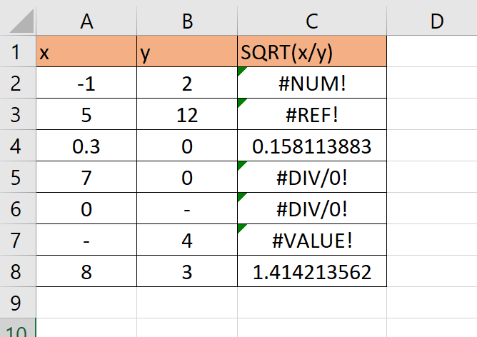
The spreadsheet below has multiple error values, including #NUM!, #REF!, and #VALUE. We can use conditional formatting and Excel functions to make the spreadsheet much less cluttered and easier to read.

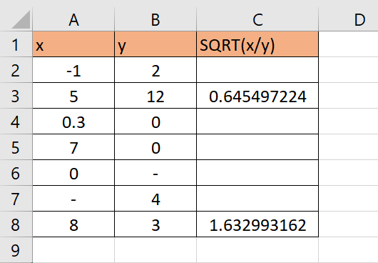
After using a custom conditional formatting rule, our table should now show a blank cell if the formula returns an error.

You can make your own copy of the spreadsheet above using the link attached below. 

If you want to try out this technique yourself in Excel, read the next section for a step-by-step guide on hiding error values.

How to Hide All Error Values in Excel

This section will guide you through each step needed to hide all error values in your Excel spreadsheet. You’ll learn how to wrap any equation with an IFERROR function to catch any potential errors. Afterward, we’ll explain how we can use conditional formatting to display blank cells.

Follow these steps to understand how to hide error values in Excel:

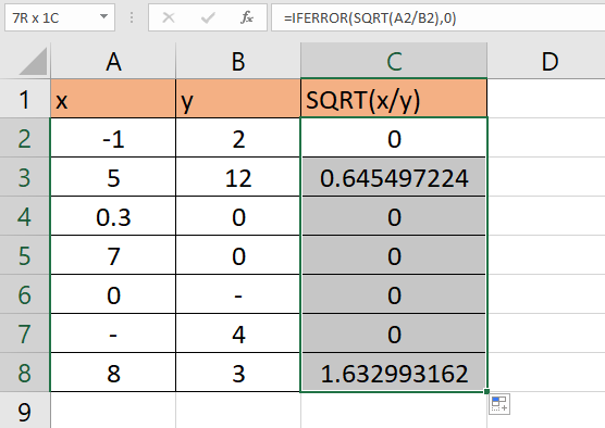
1. First, we’ll need to select the cell that may output an error. In this example, cell C2 can return an error for any number of reasons.
   For example, trying to get the square root of a negative number will result in a #NUM! error. If we divide by zero, we’ll end up with a #DIV/0! error.
   
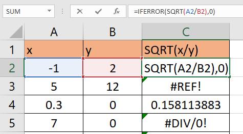
2. Next, we’ll have to wrap our main formula with an IFERROR function. In the example below, we’ve placed our main function SQRT(A2/B2) into our IFERROR function as the first argument. Our second argument will be the digit 0. This means that our formula will return 0 if the first argument causes an error.
   
3. Hit the Enter key to evaluate the function.
   
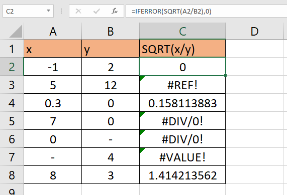
4. We can then drag down our formula to fill the rest of our column with cells that use IFERROR.
   
5. Next, select the range where you want to add conditional formatting rules. In this example, we’ve selected the cell range C2:C8.
   
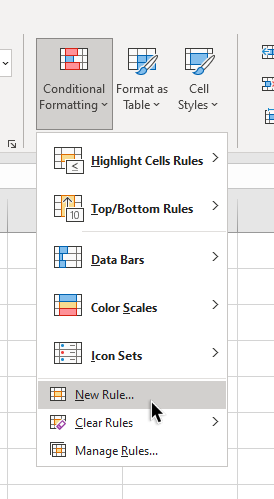
6. Look for the Conditional Formatting icon in the Home tab. Click on the New Rule… option found in the dropdown menu.
   
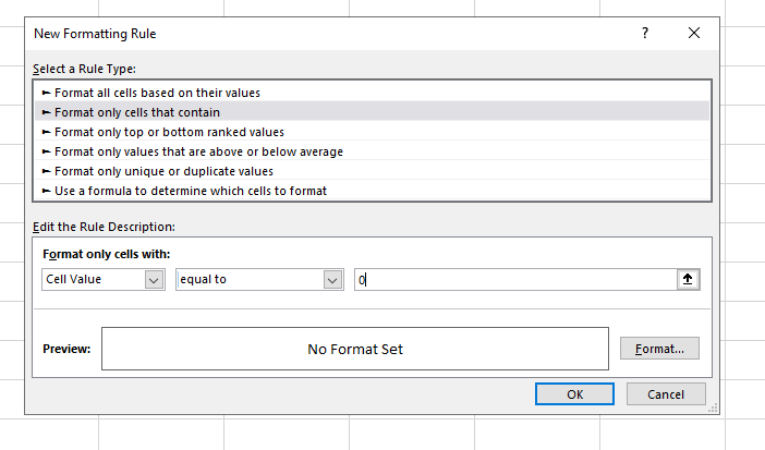
7. Select the ‘Format only cells that contain’ option as the Rule Type. For the rule description, we’d like to only format cells with a value equal to 0. Click on the Format… button to define the format used for our rule.
   
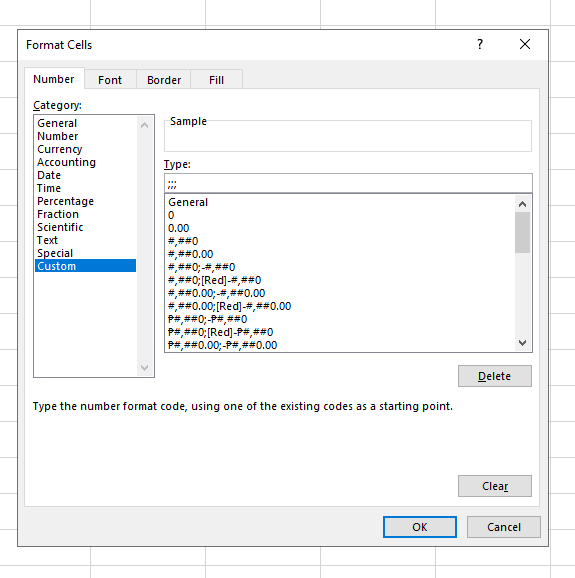
8. In the Format Cells dialog, navigate to the Number tab. Select Custom as the category.
   In the Type box, type ‘;;;’ then click on OK. The three semicolons indicate a format that hides cell values.
   
9. The final table should now hide all error values because of our custom conditional formatting rule.
   
   

Frequently Asked Questions (FAQ)

1. Can I use the IFERROR function to return my own default value?
   Yes. You can use IFERROR to return text values such as “NA”, “N/A”, “None”, or even a simple ‘-’ hyphen. You can even use an alternate formula in case the first argument returns an error.

That’s all you need to remember to start using the IFERROR function and conditional formatting together in Excel. This step-by-step guide shows how you can hide error output in your sheets easily.

The IFERROR function is another useful function in Excel that you can use to improve the overall look of your spreadsheet. With so many other Excel functions available, you can surely find one that works for you.

Are you interested in learning more about what Excel can do? 

Make sure to subscribe to our newsletter to be the first to know about the latest guides and tutorials from us.

Get emails from us about Excel.

Our goal this year is to create lots of rich, bite-sized tutorials for Excel users like you. If you liked this one, you'd love what we are working on! Readers receive ✨ early access ✨ to new content.

Subscribe