This guide will show you how you can easily highlight a cell or row with a checkbox in Excel.
Excel supports checkboxes that users can click on to manipulate values in a spreadsheet. We then use custom conditional formatting rules to highlight or stylize a cell or row based on the state of our checkbox.
Checkboxes are an interactive element in Excel that you can use to select or deselect an option. Checkboxes in Excel help users create dynamic charts, dashboards, and checklists.
Suppose you have a table in Excel where each row corresponds to a particular task or deliverable. One of the columns in this table is the ‘Done’ or ‘Approved’ field. This column has a Boolean value that can be modified through the use of a checkbox.
To make it more apparent which tasks have been accomplished, you would like to highlight tasks marked Done. How can we accomplish this?
If we want to use a checkbox to highlight a cell or row, we’ll have to use conditional formatting. Excel’s conditional formatting tool will allow us to create custom rules that will help us highlight a row if selected.
Besides highlighting the cell or row, we can also apply other formatting changes, such as striking out text or hiding it from view.
Let’s look into a working example of a table with these conditional formatting rules set up with a checkbox.
A Real Example of Highlighting Cells with a Checkbox
Let’s take a look at a real example of checkboxes that select which row to highlight.
The table below has eight columns with the last one being our checkbox. Rows where column H is checked have a green highlight while unchecked rows remain in their original format.
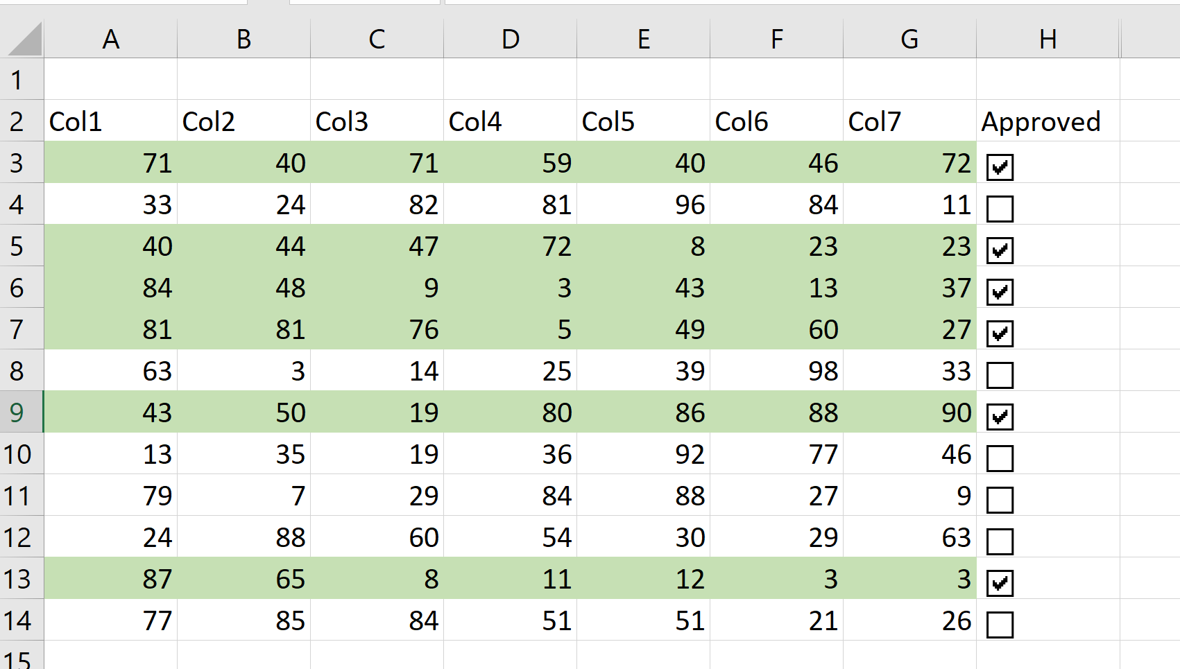
The checkbox itself does not hold the value of TRUE or FALSE. Instead, the checkboxes in column H modify a hidden column I that holds the actual Boolean value. Every time a user checks or unchecks the element, the values in column I change.
To get the right conditional formatting rules, we just need to use the following formula:
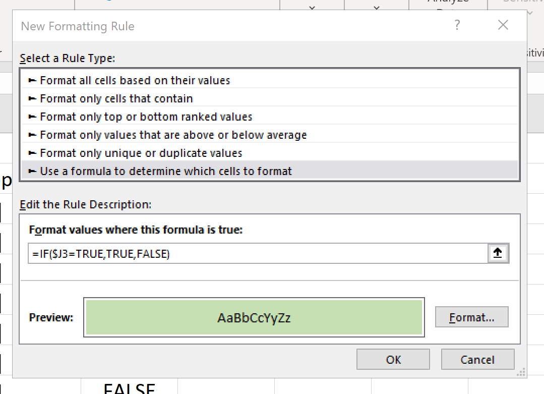
=IF($I3=TRUE,TRUE,FALSE)
Placing the ‘$’ sign before ‘I’ ensures that each cell in our range will look at column I’s equivalent cell. For example, cell B7 will have to check whether cell I7 is TRUE, and cell D12 will check cell I12. If the box is checked, then the formatting rule will take effect.
In the second example below, we used a different type of formatting for selected cells. Users can utilize the versatile formatting rules to fully customize their worksheets.

Note that if this is your first time using the checkbox in Excel, you will have to enable the Developer tab in your Excel options.
You can make your own copy of the spreadsheet above using the link attached below. Note that users can only use checkboxes in the Desktop Excel app.
Head over to the next section to learn how to do this checkbox technique on your own.
How to Use Highlight Cell or Row with a Checkbox in Excel
This section will guide you through each step needed to start using the conditional formatting rules together with checkboxes. You’ll learn how we can use custom formatting rules to change the look of an entire range of cells based on a checkbox.
Follow these steps to start highlighting cells using a checkbox:
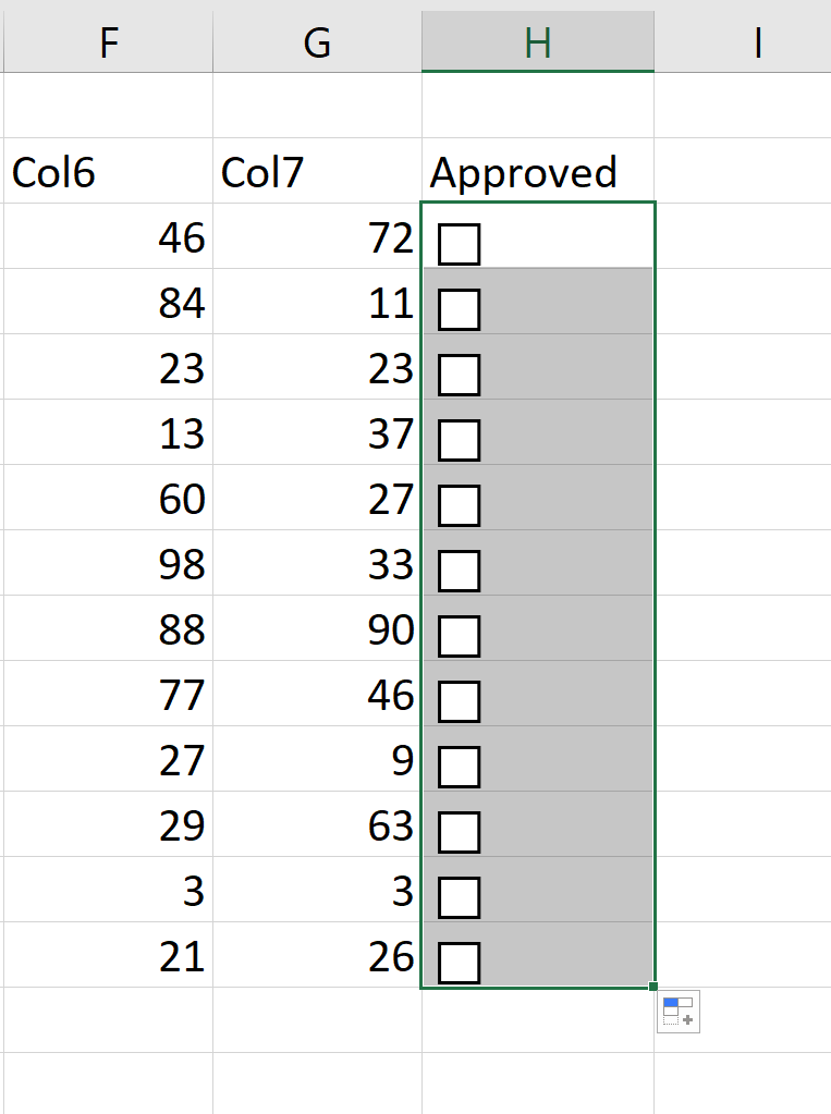
- First, we’ll need to add checkboxes to our table. You can find the checkbox element in the Developer tab under Controls -> Insert -> Form Controls.

- Next, we just have to position our checkbox over the area we want. In this example, we placed our checkbox in cell H3. You may also modify the text shown to the right of the checkbox.

- Once the checkbox is placed within a particular cell, dragging down the fill handle will also fill the additional cells with their own checkbox.
- These checkboxes do not write any values to the sheet on their own. We must link the checkbox element with a cell. Right-click on the first element and select the Format Control… option.

- In the Format Object dialog, we can select the cell to link. In this example, we’ve linked the first checkbox to cell I3.
After modifying the Cell link input, click on OK.

- Repeat steps 4 and 5 for the rest of the checkbox elements. Your table should now look like the example below.

- Now that we have a set of working checkbox elements, we can define our custom conditional formatting rules. You can find the Conditional Formatting options in the Home tab.

- Select Use a formula to determine which cells to format as the rule type. Add an IF formula to ensure that cells only change the format if their corresponding checkbox is checked.

- For formatting, you can choose whatever combination of number, font, border, and fill format options. In this example, we’ve simply added a green fill to our selected rows.
- Hit the OK button to finalize the new custom rule.
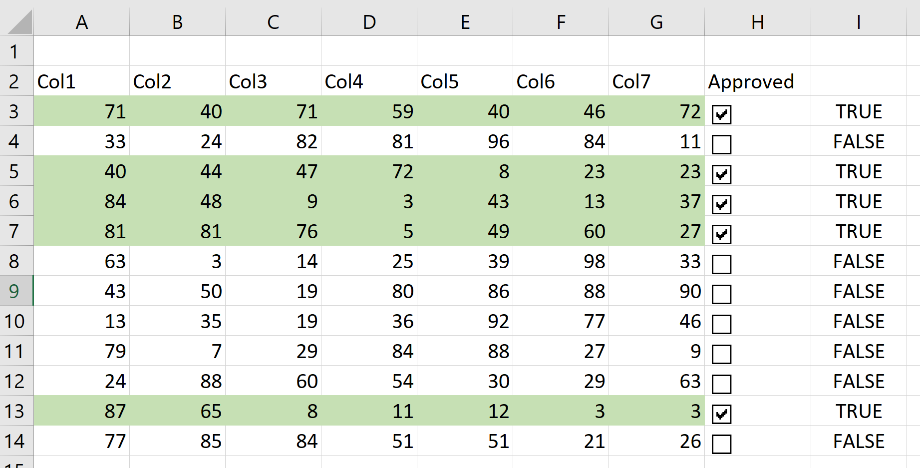
- You can hide column I since we already have a checkbox row.
That’s all you need to remember to start using checkboxes and conditional formatting to highlight rows of cells in Excel easily. This step-by-step guide shows how easy it is to apply formatting on a range based on a particular column’s value.
Conditional formatting rules is just one example of a tool in Excel that can help make your spreadsheets stand out. With so many other Excel functions out there, you can surely find a few that suit your use case.
Are you interested in learning more about what Excel can do? Make sure to subscribe to our newsletter to be the first to know about the latest guides and tutorials from us.