This guide will explain how to find the sum of multiple columns given one or more criteria.
We’ll explain how we can use the SUMIFS and SUMPRODUCT functions to find the total of all values in a given range that follows a certain condition.
Let’s take a look at a quick example where you might need to find the sum of multiple columns while following a certain set of criteria.
Suppose you have a report that keeps track of product sales. Each product has a corresponding category and sub-category. The product is also labeled by how it’s fulfilled. For example, the product may have stock in a local warehouse or be shipped overseas.
The report also further divides the report into which location sold the item. You want to determine the total revenue from all locations for a particular category.
We can use multiple SUMIF or SUMIFS functions to determine the total revenue. The SUMIFS function is helpful because it allows us to calculate the sum of all values in a certain range that meets a particular condition.
We will also explain how we can use the SUMPRODUCT function to create a more mathematical solution. SUMPRODUCT returns the sum of the products of two or more arrays. We can convert our criteria into a one-dimensional array to help filter out values in our sum range.
Now that we have a grasp on when to use the SUMIFS and SUMPRODUCT functions, let’s take a look at how they work on an actual spreadsheet.
A Real Example of Using SUMIFS on Multiple Columns with One or More Criteria
The following section provides several examples of how to use this function. We will also go into detail about the formulas and tools used in these examples.
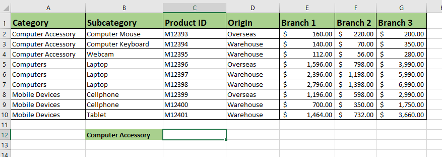
First, let’s take a closer look at our sample dataset.
The table below contains various electronics divided into three categories: Computer Accessories, Computers, and Mobile Devices.
Each product has a corresponding product ID and a field labeled ‘Origin’. The revenues for each product are split into three separate store locations.

Finding the Sum with a Single Criteria
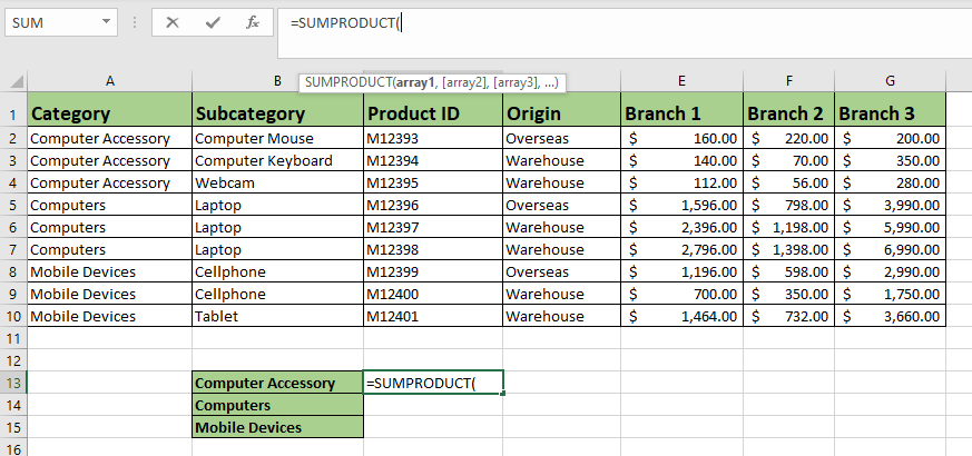
In the example below, we used the SUMPRODUCT function to get the total revenue of all computer accessories regardless of branch.

To get the total in cell C13, we just need to use the following formula:
=SUMPRODUCT($E$2:$G$10 * ($A$2:$A$10=B13))
Our SUMPRODUCT function finds the product of the range E2:G10 and the one-dimensional array A2:A10=B13. The latter range is an array with TRUE and FALSE values. The values in the range E2:G10 that are in the same row as these FALSE values are then converted to 0.
We can also make an equivalent formula that uses multiple SUMIF functions instead:
=SUMIF($A$2:$A$10;B13;$E$2:$E$10) + SUMIF($A$2:$A$10;B13;$F$2:$F$10) + SUMIF($A$2:$A$10;B13;$G$2:$G$10)
Finding the Sum with Multiple Criteria
We will have to modify our formula slightly if we need to consider more criteria. For example, suppose we also want to add the condition that the product should come from overseas.

Our SUMPRODUCT formula will need another range to multiply:
=SUMPRODUCT($E$2:$G$10*($A$2:$A$10=B18)*($D$2:$D$10=C18))
Our SUMIF function from earlier will have to be converted into multiple SUMIFS instead:
=SUM(SUMIFS($E$2:$E$10;$A$2:$A$10;B18;$D$2:$D$10;C18);SUMIFS($F$2:$F$10;$A$2:$A$10;B18;$D$2:$D$10;C18);SUMIFS($G$2:$G$10;$A$2:$A$10;B18;$D$2:$D$10;C18))
Do you want to take a closer look at our examples? You can make your own copy of the spreadsheet above using the link attached below.
Are you ready to try out the SUMIFS and SUMPRODUCT functions to get the total of multiple columns? Head over to the next section to read our step-by-step breakdown of how to do it!
How to Use SUMIFS on Multiple Columns with One or Several Criteria in Excel
This section will guide you through each step needed to start computing the sum of multiple columns given one or more conditions. You’ll also learn how we can use the SUMIF, SUMIFS, and SUMPRODUCT functions to apply a conditional sum of a range.
- First, let’s use the
SUMIFfunction to get all branches’ total revenue from computer accessories. Select the cell where you want to place theSUMIFformula. In this example, we’ll use cell C12.

- Next, we’ll fill out the arguments needed for the first
SUMIFfunction. In this example, we’ll start by usingSUMIFon the values under Branch 1.
- Use the
SUMIFfunction to get the total of the remaining columns. We’ll use the ‘+’ operation to add the results of each of these functions.
- Hit the Enter key to evaluate the function. If you want to use the Fill Handle tool, you must first convert the cell references to absolute references.

- Next, we’ll show you how to use the
SUMPRODUCTfunction to find the total of multiple columns. Select a cell and type “=SUMPRODUCT(“ to start the function.
- As an argument for
SUMPRODUCT, type the sum range and multiply it by the criteria range.
- Hit the Enter key to return the total amount.

- If you have multiple criteria, multiply the sum range by both criteria ranges.

- We can also use the
SUMIFSfunction to find the total of multiple ranges given two or more criteria.
- Each
SUMIFSfunction corresponds to two or more criteria and exactly one column. Use the SUM function to add all columns to a final result.
- Use absolute references to make it easier to use the Fill Handle tool on the formula.

This step-by-step guide should provide you with all the information you need to start using SUMIFS and SUMPRODUCT on multiple columns in Excel.
The SUMPRODUCT and SUMIFS functions are just some of the many Excel functions you can use in your spreadsheets. Our website also offers hundreds of other functions and methods to help you get more out of Microsoft Excel.
With so many other Excel functions available, you can find one appropriate for your use case.
Don’t miss out on our team’s new spreadsheet tips, tricks, and best practices. Subscribe to our newsletter to stay updated on the latest guides from us!


