


This guide will explain how you can use an Excel formula to transpose an address list from rows to columns.
We will use the ROWS, COLUMNS, and OFFSET function to build a transposed table from a single column address list.
Let’s look into a quick example of an address list that we can convert into a table.
In the example below, our address list is arranged in a single column, with each field stacked over each other. Despite not being in a table format, we can still make sense of the data by providing a few constants.
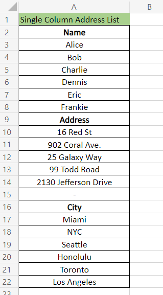
For example, we know that there are exactly three columns in the final result: Name, Address, and City. We also know that each column should have six rows, not including the header. Given these constants, we can create a formula that can transpose the data into a table.

Before we explain how you can achieve the result above, let’s look into a sample sheet that uses the formula.
A Real Example of Transposing an Address List from Rows to Columns in Excel
Let’s take a look at a real example of a sheet that converts a single-column address list into a table.
In the example below, we have an address list with three properties. Each property contains six entries. In the range D2:D4, we provided a few properties of our address list. Given these constants, we used an Excel formula to transpose the list in Column A into an actual table.
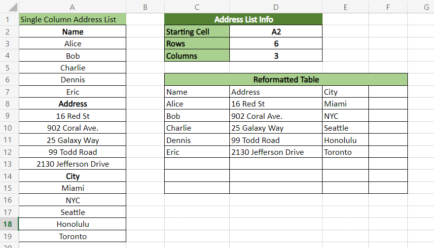
To get the table in the range C7:E12, we can use the following formula:
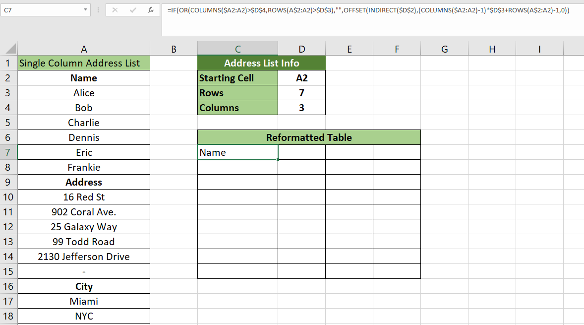
=IF(OR(COLUMNS($A2:A2)>$D$4;ROWS(A$2:A2)>$D$3);"";OFFSET(INDIRECT($D$2);(COLUMNS($A2:A2)-1)*$D$3+ROWS(A$2:A2)-1;0))
The formula above is placed in the top-left cell, and the user should drag the formula to fill out the rest of the range.
The formula first uses the IF function to check whether we should output a value. The ranges $A2:A2 and A$2:A2 increase in size due to AutoFill. If the ranges increase to a value greater than the constants provided in cells D3 and D4, the cell will return an empty string. In the example above, the cell F13 will evaluate the following formula:
OR(COLUMNS($A8:D8)>$D$4;ROWS(D$2:D8)>$D$3)
Since the number of columns in the range $A8:D8 is greater than 3, cell F13 returns an empty string.
What happens when the ranges are within the indicated bounds? This is where the OFFSET function can help us. The OFFSET function allows us to return the value of a cell that is a certain number of rows or columns away from a reference cell.
In this particular use case, our reference cell will be cell A2. Since we know that there are six rows per column, including the header, we know that adding a multiple of six will give us a different column of the same entry. Similarly, we know that we can add 1 to the row number to proceed to the next entry in a particular column.
You can make your own copy of the spreadsheet above using the link attached below.
If you’re ready to try out this OFFSET function in Excel, let’s learn how to start writing it ourselves!
How to Transpose an Address List from Rows to Columns in Excel
This section will explain each step needed to transpose a single-column address list in Excel. You’ll learn how we can convert rows to columns using the OFFSET, ROWS, and COLUMNS functions.
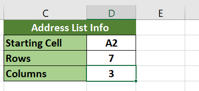
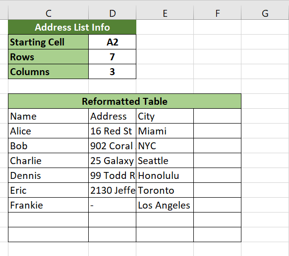
- You can follow the example below to create a dynamic sheet for transposing address lists easily. The range C1:D4 will help you set up how the formula will reformat our address list.

- Next, fill up the address list properties we need. For this example, we know that we have three columns with seven rows each. We also know that our table starts with cell A2.
- We can now add the formula shown in the previous section. Make sure that the address list information aligns with the cell references in the
OFFSETformula.

- Hit the Enter key to evaluate the formula.
- We can use the AutoFill feature by dragging the formula until the whole table is captured in the new range. Since we have a check for cells that are outside the range of our address list, we can extend the formula as much as possible.
This formula should be all you need to transpose an address list in Excel. This step-by-step guide shows how easy it is to use the OFFSET function to transpose rows to columns.
This formula is just one example of a clever way to use different functions together in Excel to manipulate data. With so many other Excel functions out there, you can surely find one that suits your use case.
Do you want to learn more about what Excel can do? Make sure to subscribe to our newsletter to be the first to know about the latest guides and tutorials from us.


