This guide will explain how to make an ANOVA table in Excel.
ANOVA tables allow users to test for statistically significant differences between data groups. By understanding how to create an ANOVA table, users can analyze their data more easily to make informed decisions.
ANOVA tables can test for statistically significant differences between groups of data. The name comes from the statistical technique ‘Analysis of variance’ that compares the means of different samples.
The goal of the ANOVA table is to help prove or disprove the null hypothesis. The null hypothesis, if true, asserts that there is no difference between the overall group means.
Let’s take a look at a simple statistical example where we might want to use an ANOVA table.
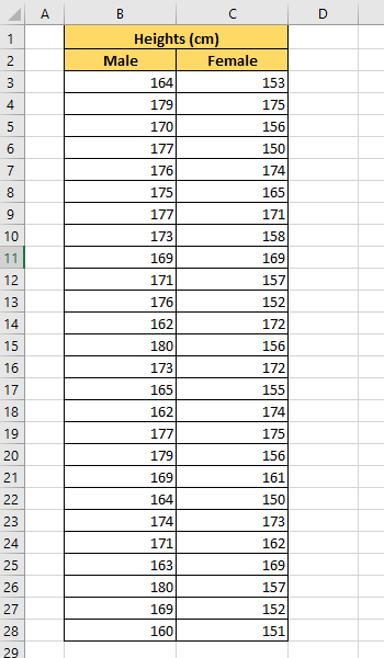
Suppose you want to test whether there is a statistically significant difference in the average heights of men and women. To do this, you would need to collect data on the heights of men and women and then input that data into an Excel spreadsheet.
After compiling the data, we can create an ANOVA table to compare the heights of each gender. We can use Excel’s Analysis Toolpak add-in to create an ANOVA table in just a few clicks.
Now that we have a grasp on when to use the ANOVA table, let’s see how this works on an actual sample spreadsheet.
A Real Example of an ANOVA Table in Excel
The following section provides several examples of how to make an ANOVA table in Excel. We will also go into detail about the formulas and tools used in these examples.
First, let’s take a look at our dataset. We have 25 samples each for both genders, with their height measured in centimeters.
The Analysis Toolpak add-in allows the user to analyze the differences between two populations quickly. The three values that are most important in the table for our purposes are the F, P-value, and F crit.

The p-value will tell you the probability that the null hypothesis is true. In other words, a low p-value indicates that the effects observed are replicable and not a result of random chance.
The higher the value of F, the higher the variation between the sample means of the different groups. However, F also takes into consideration the variation within the samples.
A low value for F indicates that the group means are close together relative to the variability within each group. The F critical value is a specific value that you can compare to the F value. You can reject the null hypothesis if F is larger than the F crit value.
Do you want to take a closer look at our examples? You can make your own copy of the spreadsheet above using the link attached below.
If you’re ready to try out making an ANOVA table, head over to the next section to read our step-by-step breakdown on how to do it!
How to Make an ANOVA Table in Excel
This section will guide you through each step needed to start using an ANOVA table to compare the sample mean of two groups. You’ll learn to use the Analysis Toolpak add-in to generate statistical measures such as the p-value and F-value.
- First, we must add the Analysis Toolpak add-in to our sheet. Click on the File tab to access the Excel Options menu.

- Click on the Options button found in the bottom-left corner of the screen.

- In the Excel Options dialog box, click on the Add-ins tab and select Go.
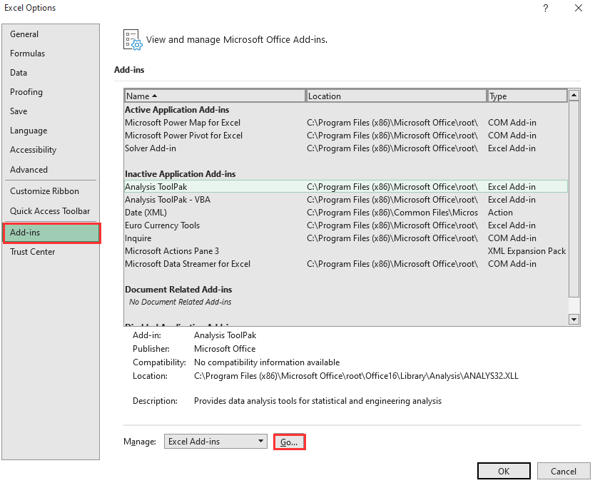
- Ensure that the Analysis Toolpak option is checked. Click on OK.

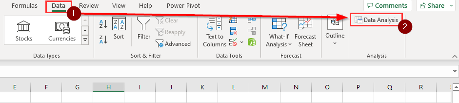
- You can find the Data Analysis option in the Data tab. Click on this option if you want to create an ANOVA table in your worksheet.
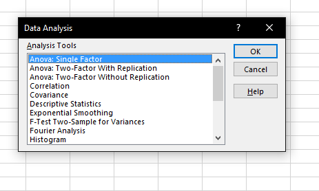
- In the Data Analysis dialog box, select the Anova: Single Factor option. Click on OK.
- For the input range, select the groups you want to compare. Select the Columns option for ‘Grouped By’ since our groups are separated into two columns.
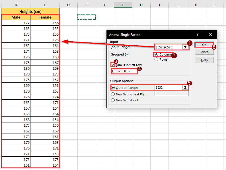
Ensure that the option ‘Labels in first row’ is checked. Set the alpha to 0.05 and provide an output range for the Anova table. Click on OK to add the table to your spreadsheet. - Your worksheet should now have an Anova table generated in the indicated output range.

This step-by-step guide should provide you with all the information you need to generate an ANOVA table in Excel.
You should now have a good idea of how the ANOVA table can help you determine the differences between two or more groups.
ANOVA is just one example of the many Excel features you can use in your spreadsheets. Our website offers hundreds of other functions and methods to help you get more out of Microsoft Excel.
For example, we can also use the Analysis Toolpak to calculate other statistical properties. You can read our guide on how we used the add-in to find the confidence interval for a given population mean.
With so many other Excel functions available, you can find one appropriate for your use case.
Don’t miss out on our team’s new spreadsheet tips, tricks, and best practices. Subscribe to our newsletter to stay updated on the latest guides from us!