How to Use KURT Function in Excel

This guide will explain how to use the KURT function in Excel.

When performing statistical analysis on a dataset, you may need to describe how heavily centered a distribution is. One way to measure this is by comparing the shape of the distribution with the normal distribution.

In statistics, kurtosis refers to the relative peakedness or flatness of a distribution compared with the normal distribution. A positive kurtosis indicates a relatively peaked distribution. Negative kurtosis indicates a relatively flat distribution.

We can use the built-in KURT function in Microsoft Excel to find the kurtosis of a given range of values. 

In this guide, we will provide a step-by-step tutorial on how to get started with the KURT function.

The Anatomy of the KURT Function in Excel

The syntax of the KURT function is as follows:

=KURT(number1,number2,...)

Let’s look at each argument to understand how to use the KURT function.

• KURT() refers to our KURT function. This function accepts one or more arguments that it will use to analyze to calculate kurtosis.
• number1 and number2 refer to the first two data points in the data set you want to find the kurtosis of.
• These arguments must be either numbers or column references that contain numbers.
• If a column reference argument contains text values, logical values, or empty values, the KURT function will ignore these invalid values. However, arguments with the value 0 are included in the calculation for kurtosis.

A Real Example of Using the KURT Function in Excel

Let’s look into a practical example where we can use the KURT function in Excel.

Suppose we have a dataset of the annual returns of a stock over the past 10 years. Each data point in the dataset refers to a given year’s annual returns (in percentages). 

We want to assess the kurtosis of these returns to understand the distribution’s shape and whether it deviates significantly from a normal distribution.

These calculations can be useful for risk assessment to understand the potential for extreme returns or losses in your investment portfolio.

To calculate the kurtosis using the KURT function, we can use the following  formula:

=KURT(A2:A11)

Our KURT formula returns the value -1.232724684 as the kurtosis value of our dataset. A negative value suggests that the distribution of annual returns is flatter than a normal distribution.

Click on the link below to create your own copy of our examples. 

Head to the next section to read our step-by-step tutorial on how to use the KURT function in Excel.

How to Use the KURT Function in Excel

1. Select the cell where you want to output the kurtosis of your given dataset.
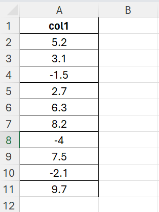
   In this example, we’ll find the kurtosis of the data points in cells A1:A11 and output the result in cell D1.
   
2. Type the KURT function and enter the cell range you want to calculate the kurtosis. We’ll use the formula =KURT(A2:A11) in this example.
   
3. Hit the Enter key to evaluate the KURT function.
   
   Our KURT function reveals that our dataset has a kurtosis of about -1.23, which indicates that the distribution of our sample has lighter tails than the normal distribution.

These are all the steps you need to know to start using the KURT function in Excel.

FAQs

1. What are the types of distributions in terms of kurtosis?
   There are three main types of distributions based on their kurtosis: mesokurtic, platykurtic, and leptokurtic. A kurtosis value of 3 indicates that our data is mesokurtic or similar to the normal distribution. Meanwhile, a value greater than 3 indicates that our distribution has heavy tails (leptokurtic). A kurtosis value less than 3 indicates a light-tailed distribution (platykurtic).
   
   
2. Why does my KURT Function return an error?
   Your function may lack arguments to calculate a proper kurtosis. If there are fewer than four data points, or if the standard deviation of the sample equals zero, the KURT function returns the #DIV/0! error value. If you encounter a #VALUE! error, one of your arguments may be a non-valid numerical value.
   
   
3. Why do we compare datasets with the normal distribution?
   The normal distribution, also known as the Gaussian distribution or the bell curve, is a common benchmark in statistics. The normal distribution has several unique properties, such as a symmetrical shape and specific tail behavior. Many forms of statistical analysis methods assume that your data follows the normal distribution. We can use the KURT function to determine whether we can assume our own data follows the normal distribution and assess whether we’ll need to adjust our statistical methods.

To learn more about using Excel for analyzing a dataset with statistics, you can read our post on how to calculate the skewness of a distribution in Excel. You may also want to read our post on how to conduct a normality test in Excel which requires you to find both skewness and kurtosis.

That’s all for this guide! Be sure to check out our library of spreadsheet resources, tips, and tricks!