How to Use LCM Function in Excel

This guide will explain how to use the LCM function in Excel.

In mathematics, the least common multiple (LCM) refers to the smallest positive integer that is divisible by a given set of two or more integers. For example, the least common multiple of 2 and 3 is 6 since 6 is the smallest number that is divisible by both factors.

Finding the LCM of certain numbers can be useful when handling recurring events. Let’s say, you have a task that happens every 10 days and another task that occurs every 6 days. We can use LCM to calculate how often these tasks occur on the same day.

With Excel, we can quickly find the least common multiple of two or more numbers with the built-in LCM function. 

In this guide, we will provide a step-by-step tutorial on how to find the least common multiple in Excel.

The Anatomy of the LCM Function

The syntax of the LCM function is as follows:

=LCM(number1, [number2], ...)

Let’s look at each argument to understand how to use the LCM function.

• LCM() refers to our LCM function. This function accepts two or more arguments for which you want to find the least common multiple.
• number1 and number2 refer to the first two data points in the data set you want to find the least common multiple of.
• The arguments must be either numbers or column references that contain numbers.
• If any of the arguments are non-numeric, LCM returns the #VALUE! error.
• If any argument is less than zero, LCM returns the #NUM! error value.

A Real Example of Using the LCM Function in Excel

Let’s explore a few simple examples where we’ll need to use the LCM function.

Using the LCM Function with Numerical Input

Suppose you wish to find the least common multiple of the integers 3 and 5. We can use the LCM function which accepts two or more integers as arguments. We can use the following formula to find the least common multiple:

=LCM(3,5)

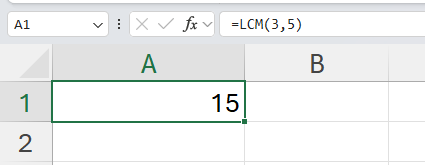
After using the LCM function, we find out that the least common multiple of 3 and 5 is 15.

Using the LCM Function with Two Cell References

In the table above, we have a dataset containing pairs of numbers representing the cycle lengths (in hours) of two connected machines. We want to identify at what cycle each pair will end at the same time. 

To find this value, we can simply look for the least common multiple of the cycle lengths of each pair of machines.

We can use the following formula to find the LCM:

=LCM(A2,B2)

In the example above, we’ve determined that the first pair of machines will finish a cycle at the same time after 180 cycles.

Using the LCM Function with Three Cell References

Let’s take a look at another example that uses the LCM function on three numbers instead.

In the table above, we are tasked to find how long it will take for each of the three machines (A, B, and C) to end at the same time. To do this, we can simply add another argument to our formula:

=LCM(A2, B2, C2)

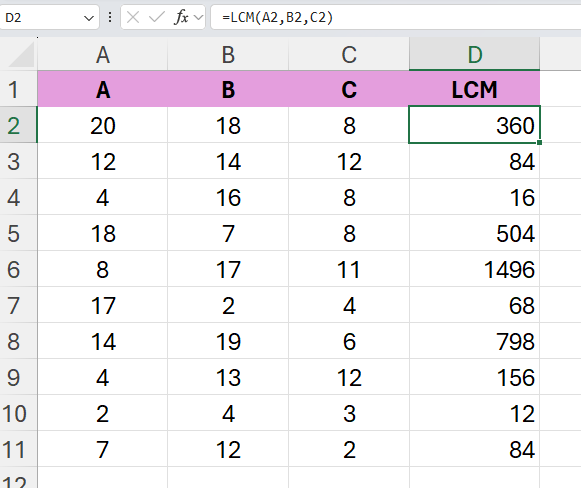
Using this revised formula, we’ve determined that the first set of machines will end at the same time every 360 hours.

Click on the link below to create your own copy of our examples.

Head to the next section to read our step-by-step tutorial on how to start using the LCM function in Excel.

How to Use the LCM Function in Excel

1. Select an empty cell and type the LCM function.
   
2. Provide at least two numerical arguments for the LCM function.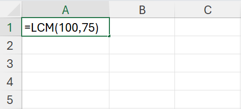
   In this example, we used the formula =LCM(100,75) to find the least common multiple of 100 and 75.
   
3. Hit the Enter key to evaluate the function. The function should return an integer that is considered the smallest common multiple of all the arguments provided.
   After evaluating our function, our formula returns a value of 300.
   
4. We can also enter cell references as arguments to the LCM function.
   In the example above, we’ll use the LCM function to find the least common multiple of each pair of values in columns A and B.

These are all the steps you need to know to start using the LCM function in Excel.

FAQs

1. Are there any limitations to the LCM function in Excel?
   The LCM function in Excel currently has a limit of up to 255 arguments. The LCM function also does not support decimal numbers. If a decimal number is provided, it will round down the number to an integer. We recommend removing the decimals using other Excel functions before finding the LCM.
   
   
2. How do I find the greatest common divisor in Excel?
   Excel also includes a GCD function that you can use to calculate the greatest common divisor of two or more numbers.
   
   
3. What happens if I provide a non-integer or non-numeric value as an argument to the LCM function?
   If the function detects a non-integer or non-numeric value, the LCM function will return a #VALUE! error.

To learn more about using Excel to help schedule events, you can read our post on how to filter dates by year in Excel.

That’s all for this guide! Be sure to check out our library of spreadsheet resources, tips, and tricks!