


The ADDRESS function is useful when you need to find the address of a named range in Excel.
This guide will explain how we can use the ADDRESS, ROW, and COLUMN functions to get a named range’s first and last cell.
A named range is used to refer to one or more cells. It is usually used to make formulas easier to parse. For example, instead of using the formula =SUM(A4:A24), we can have a formula like =SUM(Daily_Sales).
To get the scope or range of a named range, we can use the ADDRESS function. Let’s take a look at a quick example!
Suppose we have a table with employee data, including first name, last name, and email. The entire table has been assigned the name ‘EmployeeTable’. Given the named range, is it possible to get the full address?

To get the full address, we’ll require the location of two cells: the cell in the top-left corner and the cell in the bottom-right corner. For example, if we know that the top-left cell is A2 and that the bottom-right cell is D3, then the range’s full address is simply A2:D3.
How can we obtain these two key cells? Excel has an ADDRESS function that returns the address of a specific row and column. We can use this function alongside the ROW and COLUMN functions to calculate the first and last cells.
Now that we know what functions to use, let’s explore how the mentioned functions are used to create a formula to get the address of a named range.
A Real Example of Obtaining the Address of Named Range in Excel
Let’s take a look at a real example of a formula that allows us to get the address of a named range in an Excel spreadsheet.
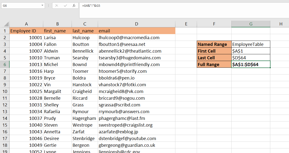
To get the address of our employee table, we first compute the location of the first cell in cell G4. Next, we’ll locate the address of the last cell in the named range in cell G5. We can now simply concatenate these values to get the full address.
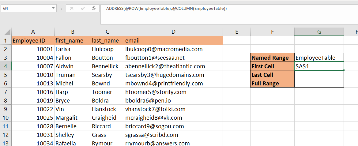
To get the first cell, we just need to use the following formula:
=ADDRESS(@ROW(EmployeeTable),@COLUMN(EmployeeTable))
In this example, the arguments @ROW(EmployeeTable) and @COLUMN(EmployeeTable) both return 1. The ADDRESS function outputs the cell found in the first row and first column, which is cell A1.
To get the last cell, we can use the following formula:
=ADDRESS(@ROW(EmployeeTable)+ROWS(EmployeeTable)-1,@COLUMN(EmployeeTable)+COLUMNS(EmployeeTable)-1)
This formula gets the last cell by finding the row and column of the cell in the bottom–right corner of the range. To get the row of this last cell, we simply add the number of total rows in the range to the row number of the first cell. Similarly, we add the total number of columns to the column number of the first cell.
To get the final address, we use this simple formula:
=G4&":"&G5
You can make your own copy of the spreadsheet above using the link attached below.
If you’re ready to try out the formulas yourself in Excel, follow the guide in the next section!
How to Get Address of Named Range in Excel
We will now guide you through how to start using the ADDRESS function in Excel to get the full address of a named range. You’ll learn how we can use the ROW and COLUMN functions to locate the first and last cells of the named range.
Follow these steps to get the address of named ranges in Excel:
- First, identify which named range you would like to find the address of. In this example, we’ll get the full address of the named range EmployeeTable.
 To find a list of named ranges, you can type in the shortcut Ctrl+F3, or you can click on the Name Manager option in the Formulas tab.
 - Next, we’ll use the
ADDRESSformula for calculating the first cell in the range. Simply input the named range into theROWandCOLUMNfunctions.
- Use the
ADDRESSformula for getting the last cell in the named range.

- After obtaining the first and last cell of the range, we can create the full range by concatenating both values. We’ll have to add a colon character ‘:’ between both values.
Frequently Asked Questions (FAQ)
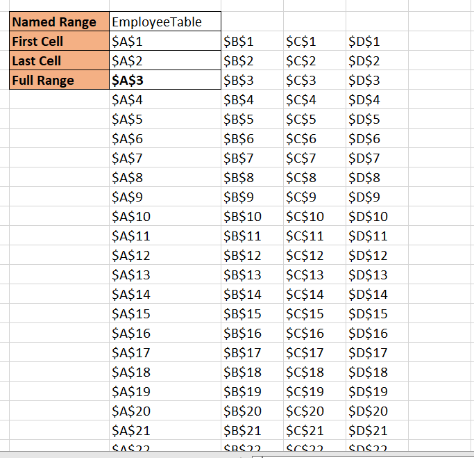
- Why does my formula require an ‘@’ symbol?
The ‘@’ symbol is used in Excel as the implicit intersection operator. It is typically used to force a cell to return a single value. Since a named range is used as an argument to theROWandCOLUMNfunctions, the formula would return a range like in the spreadsheet below.
This guide has explained everything you need to start using the ADDRESS function to get the address of a named range in Excel. We’ve learned how we can use the ROW and COLUMN functions to get the boundaries of a named range and use the results to return the final address.
You can now use these functions in Excel together with the various other Excel formulas available to create great worksheets that suit your problem.
Are you interested in finding out more about what Excel can do? Make sure to subscribe to our Excel newsletter to be the first to know about the latest guides and tutorials from us.


