This guide will explain how to calculate the Spearman rank correlation in Excel.
This calculation is helpful if you want to analyze the relationship between two ranked variables.
Spearman rank correlation is a statistical measure of the relationship between two ranked variables. The CORREL function can be used to calculate the spearman rank correlation in Excel. The t-statistic and p-value can be used to determine whether the spearman rank correlation is statistically significant.
Let’s take a look at a simple example where we can calculate spearman rank correlation.
We can use the Spearman rank correlation method to determine the relationship between age and body mass index. If there is a positive correlation, then this indicates that someone’s BMI increases as they grow older.
After finding the correlation. We’ll use other statistical techniques to determine whether there is a statistically significant relationship between the two variables.
Now that we know when to use the calculate spearman rank correlation function, let’s see how this works on an actual sample spreadsheet.
A Real Example of Calculating Spearman Rank Correlation in Excel
The following section provides several examples of how to calculate Spearman rank correlation in Excel. We will also go into detail about the formulas and tools used in these examples.
First, let’s take a closer look at our sample dataset. Each row in our dataset corresponds to a single person chosen randomly from a population. We have data on their age in years as well as their body mass index value or BMI.
![]()
We can use the RANK function to return the rank of each value in both rows. We’ll perform this operation for both fields.
![]()
Once we have the rankings of every value, we can use the CORREL function to find the Spearman correlation coefficient.
![]()
We’ll use the following formula to find the Spearman correlation coefficient:
=CORREL(D4:D14;E4:E14)
The CORREL function’s two arguments are cell references to the two ranking columns we generated earlier.
After finding the Spearman correlation coefficient, you may want to determine the measurement’s p-value. The p-value indicates how likely your data may have occurred by a chance.
![]()
A p-value lower than 0.05 is a sign that your result has statistical significance. We used the TDIST function to calculate the p-value given size of the sample and the t-statistic.
Do you want to take a closer look at our examples? You can make your own copy of the spreadsheet above using the link attached below.
Use our sample spreadsheet to take a closer look at the statistical functions we used to find the t-statistic.
If you’re ready to try out calculating Spearman rank correlation, head over to the next section to read our step-by-step breakdown on how to do it!
How to Calculate Spearman Rank Correlation in Excel
This section will guide you through each step needed to find the Spearman rank correlation of two variables in Excel.
Follow these steps to start using the Spearman rank correlation function.
- First, we will need to create two new columns. These columns will provide a ranking for each value in both fields we are trying to measure.

- We’ll use the
RANK.AVGfunction to determine the current age’s rank against the set of sample ages. The third argument is set to ‘1’ to indicate that we want to rank these values in ascending order.
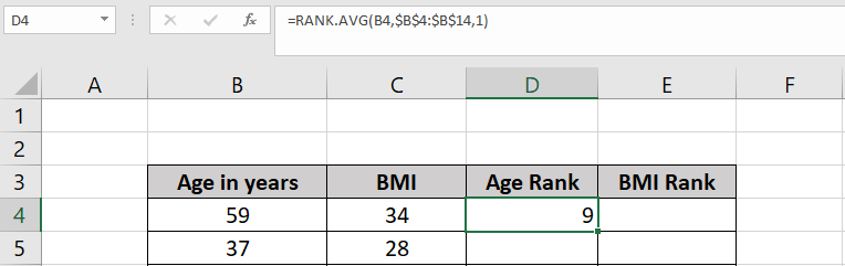
- Proceed to do the same for the BMI values.

- Use the Fill Handle tool to calculate the ranking of every value from both fields.

- Use the
CORRELfunction to find the Spearman correlation coefficient.

- Hit the Enter key to return the final result.

- To find the p-value of our correlation, we’ll first have to compute for N and the t-statistic. The value of N is simply the size of our sample. The T-statistic is calculated using the formula
=(ABS(H3)*SQRT(H4-2))/(SQRT(1-ABS(H3)^2)).

- After finding these values, we can calculate the p-value using the formula
=TDIST(H5;H4-2;2).

These are all the steps needed to calculate the Spearman rank correlation in Excel.
Frequently Asked Questions (FAQ)
- How do I interpret Spearman rank correlation?
A Spearman rank correlation of -1 indicates a perfect negative correlation, meaning that as one variable increases, the other decreases. A Spearman rank correlation of 1 indicates a perfect positive correlation, meaning that as one variable increases, the other also increases. A Spearman rank correlation of 0 indicates no correlation between the two variables.
This step-by-step guide should provide you with all the information you need to calculate the Spearman rank correlation in Excel
This statistic can help determine whether there is a correlation between two different variables in a given population. A positive Spearman rank correlation suggests that increasing one variable will also increase the other.
Calculating Spearman rank correlation is just one example of the many statistical methods you can use in your Excel spreadsheets. Our website offers hundreds of other functions and methods to help you get more out of Microsoft Excel.
With so many other Excel functions available, you can find one appropriate for your use case.
Don’t miss out on our team’s new spreadsheet tips, tricks, and best practices. Subscribe to our newsletter to stay updated on the latest guides from us!