How to Use the TOROW Function in Google Sheets

This guide will explain how to use the TOROW function to convert an array or range of cells into a single row.

Suppose you have an array of values in a 9×9 range of cells in your spreadsheet. You want to display all these values as a single row rather than a two-dimensional array.

We can use the TOROW function in Google Sheets to convert our range into a single row quickly.

In this guide, we will provide a step-by-step tutorial on how to begin using the TOROW function. We will cover how to adjust the parameters of the function to control how the function handles errors and blank cells.

Let’s dive right in!

The Anatomy of the TOROW Function

The syntax of the TOROW function is as follows:

=TOROW(array_or_range, [ignore], [scan_by_column])

Let’s look at each argument to understand how to use the TOROW function.

• = the equal sign is how we start any function in Google Sheets.
• TOROW() refers to our TOROW function. This function accepts an array or range and outputs the values as a single row.
• array_or_range refers to the array or range of cells you want to return as a single row.
• The [ignore] parameter allows us to specify what values to ignore. By default, this value is 0, which means all values are kept. A value of 1 sets the formula to ignore blanks. Specifying a value of 2 ignores all errors. A value of 3 makes the function ignore all blanks and errors. 
• [scan_by_column] is a boolean value that determines how the function scans the array. Setting the value to True will make the function scan the array by column. Setting the value to False will make the function scan by row instead.

A Real Example of TOROW Function in Google Sheets.

Let’s explore a simple example where we may need to use the TOROW function in Google Sheets.

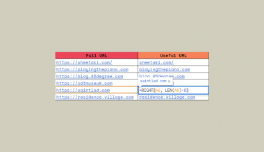
In the table seen below, we have a list of names separated into three different columns.

In another part of our sheet, we want to create a new table where each name is a column header. This setup requires each name to be placed in a single column.

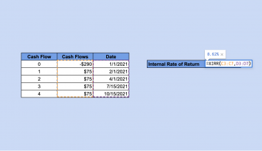
We were able to return the output in row 6 using the following formula in cell B6:

=TOROW(A2:C4, 1, TRUE)

The formula above generates the new row by going through each column of the range, starting from the leftmost column. After entering the formula in cell B6, the output spills automatically into as many cells as needed to hold all the values in the range.

If we use the formula =TOROW(A2:C4, 1, FALSE), our output will follow the order of values starting from the top-most row instead.

Do you want to take a closer look at our examples? You can make your own copy of the spreadsheet above using the link attached below. 

Use our sample spreadsheet to see how adjusting the parameters of our function affects the output.

If you’re ready to try using the TOROW function yourself, head over to the next section to read our step-by-step breakdown on how to do it!

How to Use the TOROW Function in Google Sheets

This section will guide you through each step needed to use the TOROW function in your Google Sheets spreadsheet. We will also explain how to control how the function handles errors and blank cells.

Follow these steps to convert a range into a single row:

1. First, select an empty cell in your spreadsheet and type “=TOROW(“ to begin the TOROW function.
   
   
2. For the first argument, enter the range you want to convert into a single row.
   In our example above, we want to output the list of names in A2:C4 into a list of names in row 7.
3. We can now hit the Enter key to evaluate the TOROW function. By default, the function will follow the order of values from left to right, starting from the top-most row.
   
   
4. By default, blank cells are still included in the output.
   
   
5. We can skip the blank cells in the output by setting the second parameter to 1.
   
   
6. If we set the third argument to TRUE, our output will follow the order from top to bottom, starting from the left-most column.
   

Frequently Asked Questions (FAQ)

Here are some frequently asked questions about this topic:

1. How do I make the TOROW function return only unique values?
   We can combine the UNIQUE and TOROW functions to output all unique values in a range as a single row. For example, the formula =UNIQUE(TOROW(A2:C4), TRUE) will return all unique values in the range A2:C4 as a single row. We need to set the second argument of UNIQUE to TRUE to allow it to find duplicates within a row rather than within a column.

This tutorial should cover everything you need to know to start using the TOROW function in Google Sheets.

We’ve explained how to use the TOROW function to output a range of values into a single row.

The TOROW function is just one example of a built-in Google Sheets function you can use to manipulate your data. Another function that might be useful is the TRANSPOSE function. You can read our guide to learn how to use the function to swap rows to columns and vice versa.

You may also check our guide on how to use the HSTACK function in Microsoft Excel to learn more about combining multiple arrays horizontally.

That’s all for this guide on the TOROW function! If you’re still looking to learn more about Google Sheets, be sure to check out our library of Excel resources, tips, and tricks! 

Get emails from us about Excel.

Our goal this year is to create lots of rich, bite-sized tutorials for Excel users like you. If you liked this one, you'd love what we are working on! Readers receive early access to new content.

Subscribe