This guide will explain how to transpose data in Excel using three simple and easy methods.
Excel is a popular tool that is extremely useful for different kinds of tasks. For example, inputting data, performing analysis, making reports, and calculations. And all of these tasks require data.
But what should we do if our needed data needs to be pasted differently? Worry not!
Because Excel can transpose data from one column or row to another column or row in the worksheet, we do not have to worry about this issue at all. And this is why Excel is such a useful tool.
Let’s take an example wherein we need to transpose data in Excel.
Suppose you have a monthly sales report containing the stores and their sales. And doing this entire process with a very large data set manually would take too much time and is simply inefficient.
Great! Now let’s move on and discuss how to transpose data in Excel using three easy and simple methods.
The Anatomy of the TRANSPOSE Function
The syntax or the way we write the TRANSPOSE function is as follows:
=TRANSPOSE(array)
Let’s take apart this formula and understand what each term means:
- = the equal sign is how we start any function in Excel.
- TRANSPOSE() is our
TRANSPOSEfunction. And this function will convert any vertical range of cells to a horizontal range, or vice versa. - array is the only argument needed. And this refers to the range of cells or array of data we want to transpose.
How to Transpose Data in Excel using TRANSPOSE function
Firstly, we can utilize the TRANSPOSE function method to transpose data in Excel. From the name itself, the TRANSPOSE function automatically transposes the data for us.
To do this, follow the steps below:
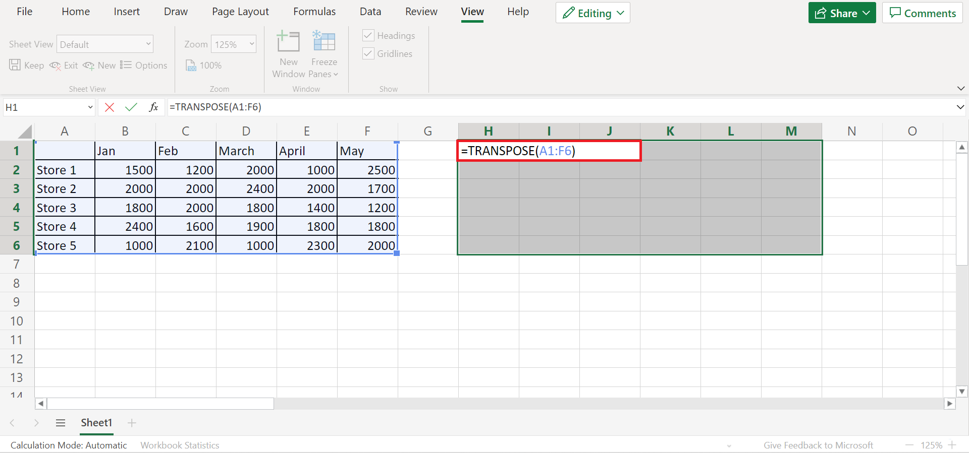
1. Firstly, we need to select a range of cells where we will transpose the data set. And make sure this range is the exact size of the original dataset. Then, start the TRANSPOSE function in the top left cell. So type in the formula “=TRANSPOSE(A1:F6)”. Lastly, click on the Enter key to transpose the data set.
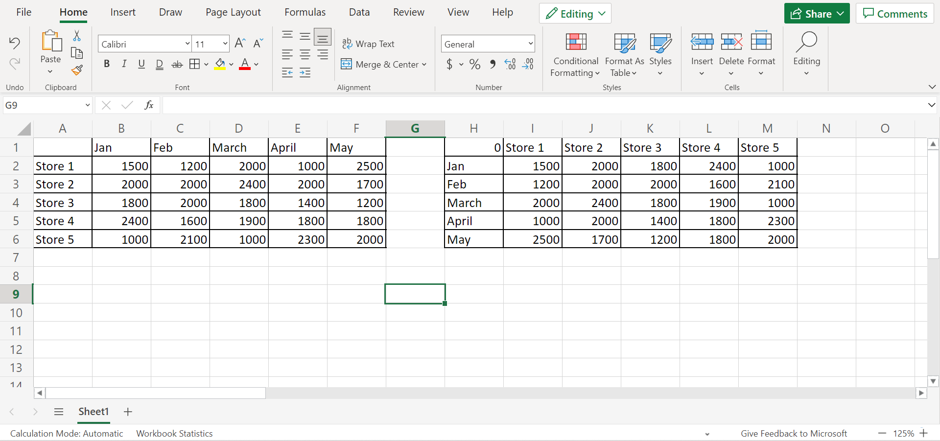
2. And tada! We have successfully transposed data in Excel using the TRANSPOSE function.
How to Transpose Data in Excel using Paste Transpose
Secondly, we have the method to use the paste transpose feature. So the paste transpose feature can immediately transpose our data set.
For instance, our data set is arranged so that the stores are in a column while the months are in a row. But, we need to switch or transpose the arrangement for some reason. And this is where the paste transpose feature comes in.
To use the paste transpose feature to transpose data in Excel, follow the steps below:
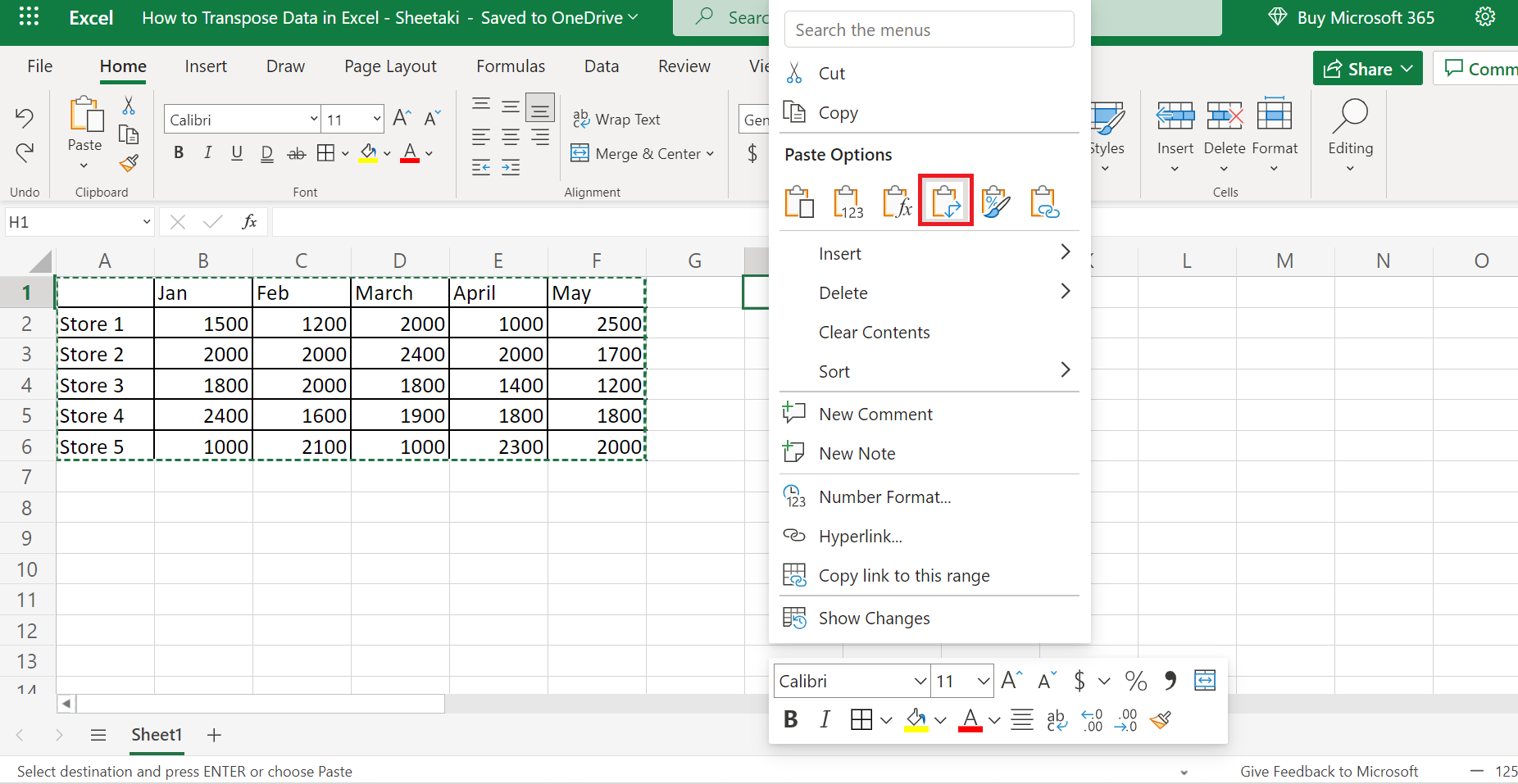
1. Firstly, we need to select our entire data set. In this case, we will select the range A1:F6 which contains our data.

2. Secondly, we need to copy the data set. To copy, we can press the Ctrl + C keys. And we can also right-click and select Copy.

3. Then, we can paste the copied data set into another location. In this case, we will paste the data set in range H1:M6 . So right-click on the cell and click Paste Transpose.
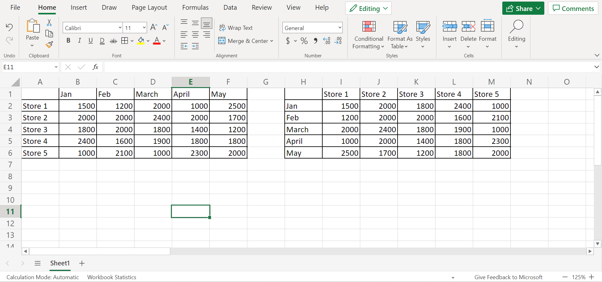
4. And tada! We have successfully transposed the data set. So now the stores are in a row while the months are in a column.

How to Transpose Data in Excel using Paste Special and Find & Replace features
And the third method to transpose data in Excel is using a combination of the paste special feature and the find & replace feature. So one thing to note about using the paste special method is that it gives us a static data.
And this means that any changes we make in the original data set will not reflect or update in the transposed data set. So we would have to perform the entire process again.
But this would take time to do. So the second method would ensure that when we transpose our data set, it would still be linked to the original data set.
To learn how to do the second method, follow the steps below:
1. Firstly, we must select our data set in range A1:F6.
2. Secondly, we will copy the selected data set. To copy it, press Ctrl + C or right-click and select Copy.

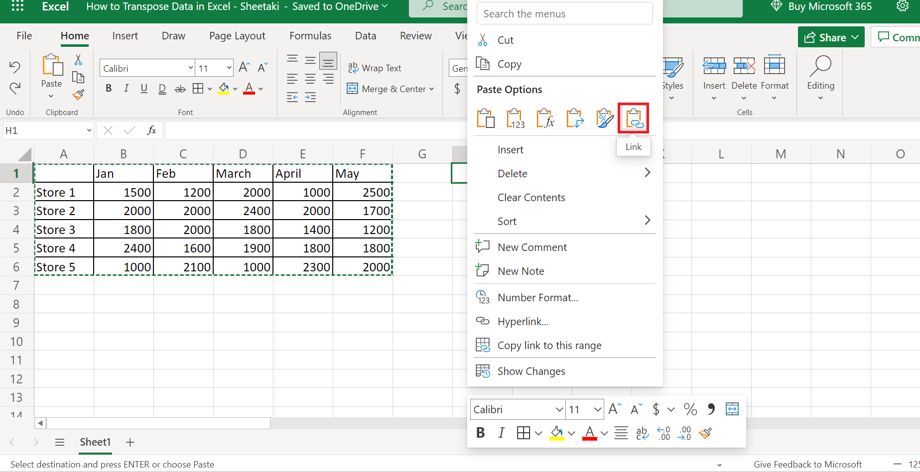
3. Then, we can now paste the copied data set into another location. In this case, we will paste in at range H1:M6. So right-click the cell and select Paste Link.
4. Afterward, we will copy this data set again. So right-click and select Copy or click the Ctrl + C keys.

5. Then, we will paste the data set into another location. Again, right-click and select Paste Transpose.

6. And tada! We have transposed our data set. Furthermore, we can make changes in the original data set and reflect them in the transposed data set.
You can make your own copy of the spreadsheet above using the link attached below.
And that’s pretty much it! We have discussed how to transpose data in Excel using three simple and easy methods. Now you do not have to worry about manually retyping your data set. So you can simply choose any of the three methods and transpose your data set immediately when needed.
Are you interested in learning more about what Excel can do? You can now use the TRANSPOSE function and the various other Microsoft Excel formulas available to create great worksheets that work for you. Make sure to subscribe to our newsletter to be the first to know about the latest guides and tutorials from us.