This guide will explain how to use the VLOOKUP function for exact matches in Excel.
VLOOKUP is a great way to search for a specific value in a dataset. The VLOOKUP function allows users to get data from a table by matching a lookup value with values on the leftmost column of the table.
For example, given an employee’s ID number, we can use VLOOKUP to find a match in a lookup table and output details such as the employee’s name and department.
However, you may not realize that the VLOOKUP function assumes your values are sorted in ascending order. And by default, it does not look for an exact match but rather an approximate match.
In this guide, we will provide a step-by-step tutorial on how to use the VLOOKUP function to find exact matches. We will also cover how to modify the VLOOKUP function to handle case-sensitive searches.
A Real Example of Using VLOOKUP Function with Exact Match in Excel
Let’s explore a sample spreadsheet where we’ll need to use VLOOKUP to find an exact match.

In the table above, we have a lookup table containing country codes and their corresponding country name. For example, the country code ‘AU’ refers to the country of Australia.
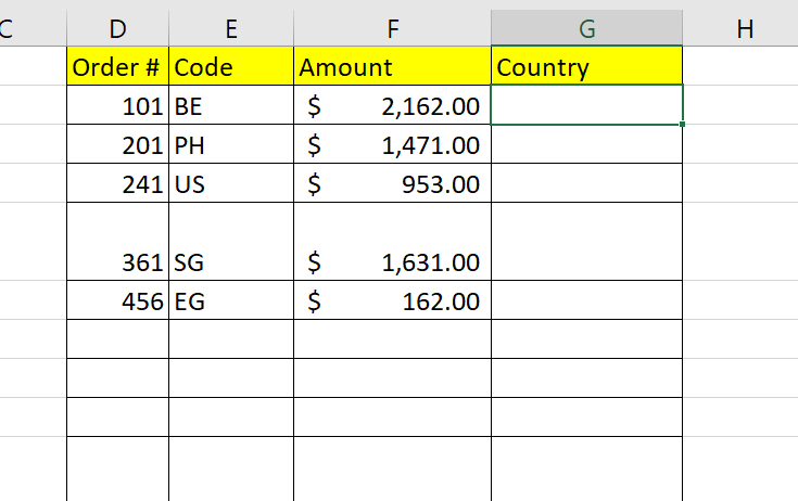
In a separate table, we are keeping track of various international orders. Each order has an order number, the country code of where the order was placed, and the total order amount. We want to fill out a fourth field labeled Country with the full name of the country based on the order’s country code.

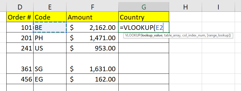
Since we already have a lookup table for country codes and country names, we can search for country names using the VLOOKUP function. We can find the country name from a given country code using the following formula:
=VLOOKUP(E2,A:B,2,FALSE)
In the above formula, we are searching for the value in cell E2 (“BE”) in the range A:B and returning the value in the second column. The “FALSE” parameter indicates that we only want exact matches.

We’ll add our formula to column G so that the column will display the full name of the country based on the country code written in column E.
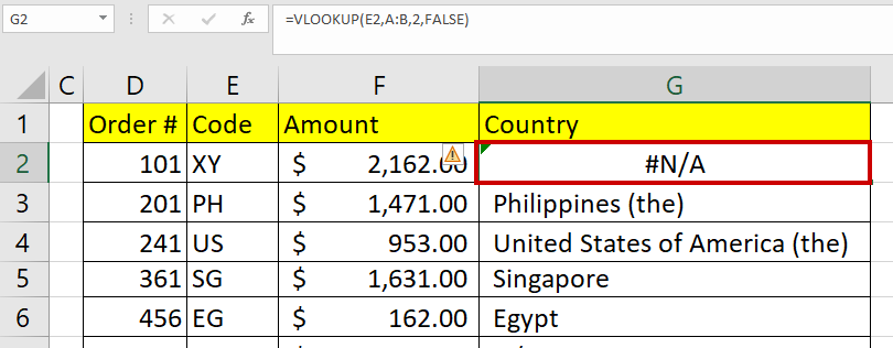
If no exact match is found, our formula will return a #N/A error instead. We can further modify our formula to handle these errors.

In the image above, the IFNA function is used to catch potential #N/A error values and return custom text instead. These #N/A errors occur when the lookup value can’t be found in the leftmost column of the provided range.
We’ll use the following formula to return the text “N/A” when an exact match is not found:
=IFNA(VLOOKUP(E2,A:B,2,FALSE),"N/A")
Finding a Case-Sensitive Exact Match
A downside of the VLOOKUP function is that when finding exact matches, the function disregards differences in lowercase and uppercase letters. For example, the lookup values “BE”, “bE”, and “be” will return the same result.
If your use case requires a case-sensitive search, we can modify the VLOOKUP formula:
=IFNA(VLOOKUP(TRUE,HSTACK(EXACT(A:A,F2),B:B),2,0),"N/A")
To understand the formula, let’s take a closer look at the functions used within it. The EXACT function takes two arguments and returns TRUE if the two arguments are an exact match (case-sensitive). Otherwise, the formula returns a FALSE value.

In the example above, we have a small subset of country codes and country names. We can see that the formula in cell L7 returns FALSE because “BE” is not an exact match to the lookup value “bE” in cell K2.
Next, we’ll use the HSTACK function to combine the country names with the results of the EXACT function.
The HSTACK function takes two arrays as arguments, joins them horizontally, and returns the output. This joined array will serve as our lookup table in the VLOOKUP function.

In the image above, we used the formula =HSTACK(EXACT(J5:J8,K2),K5:K8) to combine the results of our EXACT function and the corresponding country name. Instead of using VLOOKUP to search for country codes directly, we will simply look for the first row in our HSTACK output with a TRUE value.

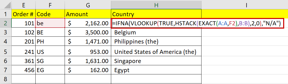
In the table above, orders with an incorrect case (“be”) receive an output of “N/A” since our EXACT function will not return any TRUE values. However, using the proper case (“BE”) will output the correct result.
Here’s the formula we used in column H:
=IFNA(VLOOKUP(TRUE,HSTACK(EXACT(A:A,F2),B:B),2,0),"N/A")
Click on the link below to create your own copy of our examples.
Head to the next section to read our step-by-step tutorial on how to use VLOOKUP to find exact matches.
How to Use VLOOKUP Function with Exact Match in Excel
- Select the first cell you want to add the
VLOOKUPfunction to.
- Type “=VLOOKUP(“ to start the function. Select the cell that contains the lookup value you want to search for.
- Next, enter a reference to the table array you want to search through for the lookup value.

- For the third argument, enter the index of the column you want to return if a match is found. Add FALSE as the fourth argument to ensure that we will only find exact matches.

- Hit the Enter key to evaluate the
VLOOKUPfunction.

- We can use the Auto-Fill feature to apply the same formula to the rest of column G.
 Use your cursor to drag the first cell’s Fill Handle downward to copy the
 VLOOKUPformula.
- We can wrap our
VLOOKUPfunction with anIFNAfunction to handle cases where the lookup value cannot be found.
 In our example above, we used the formula =IFNA(VLOOKUP(E7,A:B,2,FALSE),”N/A”).
- We can modify our
VLOOKUPformula to perform a case-sensitive search for exact matches. We’ll use the formula =IFNA(VLOOKUP(TRUE,HSTACK(EXACT(A:A,F2),B:B),2,0),”N/A”)
 The formula HSTACK(EXACT(A:A,F2),B:B) will create a range with two columns. The first column is only equal to TRUE when a row’s country code matches the case of the lookup value in F2. The second column is the corresponding country name of each country code.
You should now have an in-depth understanding of how to use VLOOKUP to find exact matches. To learn more about using VLOOKUP, you can read our post on how to use VLOOKUP using a given time range.
That’s all for our guide! Be sure to check out our library of spreadsheet resources, tips, and tricks!