


This guide will discuss how to display numbers as fractions in Excel using two simple and efficient ways.
Excel is an excellent tool for inputting numbers and calculations. But, there is one thing Excel does that may be frustrating sometimes. And this is when Excel changes the format of inputted numbers.
For instance, Excel usually converts the fractions we input into decimals, numbers, or other number formats. And this can be annoying if we want to display them as fractions.
In mathematics, a fraction is a numerical quantity that represents the parts of a whole. But, fraction in Excel is a type of number format.
So an explanation could be because fractions are not one of the data types Excel supports or understands. Because it cannot understand it, Excel will try to convert it to a data type it understands, such as into a text string or decimals.
Let’s take an example wherein this issue may occur.
Suppose you are inputting data into an Excel worksheet. And your data happens to contain fractions. But, you noticed that once you finish typing in your fractions, it converts into a date instead.
Worry not, though! We will be discussing simple and quick ways how to display numbers as fractions in Excel. But first, let’s check out a real example of how to display numbers as fractions in Excel.
A Real Example of Displaying Numbers as Fractions in Excel
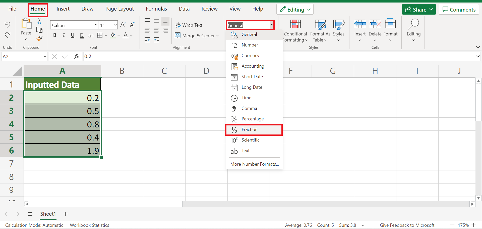
Let’s say we have data from our research containing fractions. But, as we continue to input the data, we notice that Excel converts them into a different data type. In this case, our inputted data gets converted into decimals and would look like this:

Then, we can apply two methods to display the data as fractions instead. Firstly, we can simply change the number format to a fraction. And tada! We have displayed the numbers as fractions.
Another way we can use it is by applying a custom format. And this method is best used if our data is not a simple fraction but instead is a mixed fraction. Because we can choose many custom formats to display the fraction correctly, this method is recommended for those types of fractions.
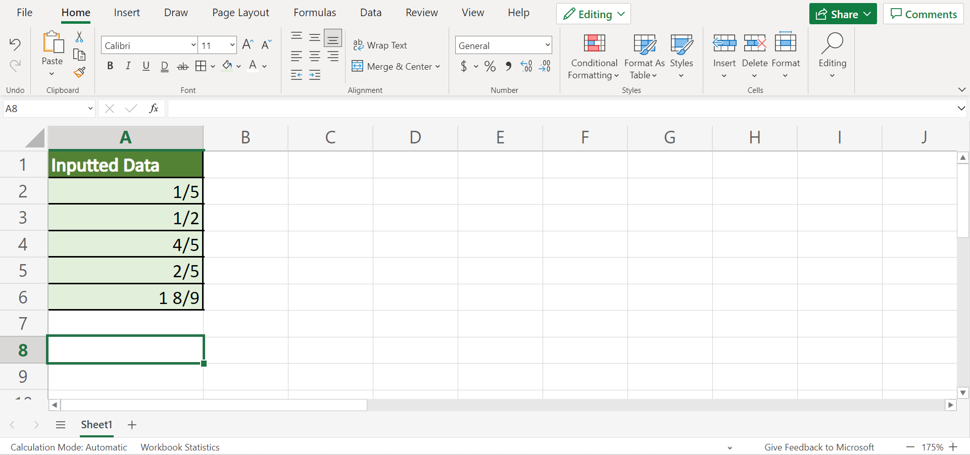
Finally, our final output would look like this after displaying the numbers as fractions in Excel:

You can make your own copy of the spreadsheet above using the link attached below.
Awesome! Now let’s start learning the two simple and efficient methods of how to display numbers as fractions in Excel.
How to Display Numbers as Fractions in Excel by Changing the Number Format
The first method to display numbers as fractions in Excel is simply changing the number format.
To learn this method, let’s follow the steps below:
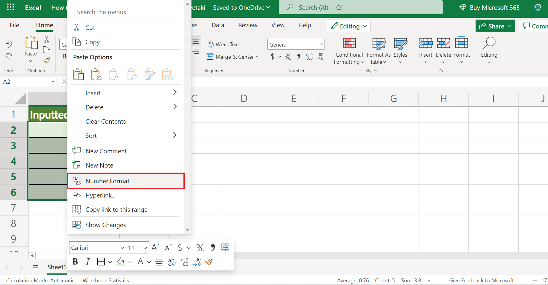
1. Firstly, we need to select the cell containing the number we want to change the format to a fraction. Then, right-click and select Number Format.

2. Secondly, the Number Format will appear. Under Category, select Fraction and choose a Type of your preference. Lastly, click OK to apply the changes in the format.

3. And tada! We have successfully displayed the numbers as fractions in Excel.
4. Alternatively, we can also go to the Home tab and click the Number Format dropdown menu. Then, select Fraction to convert the number.
How to Display Numbers as Fractions in Excel by Applying Custom Format
The second method we can use is an extension of the first method. Because Excel allows its users to customize number formats, we can utilize this feature and create a custom format to convert numbers as fractions.
Furthermore, it can be confusing at first to understand what the symbols in the custom format mean. So here is a table to guide you along what each symbol can mean.
| Format | Description |
| # ?/? | A mixed fraction up to a single digit denominator |
| # ??/?? | A mixed fraction up to a double-digit denominator |
| ???/??? | An improper fraction up to a three-digit denominator |
| # ??/256 | A mixed fraction with a fixed denominator of 256 |
To do this method, let’s discuss the step-by-step process below:
1. Firstly, select the cell containing the numbers you want to convert into fractions. Then, right-click and select Number Format.
2. Secondly, the Number Format window will appear. In this window, go to the Custom category. Then, we can input a custom format in the space below Type:. For instance, we will choose “# ?/?” for a mixed fraction. Lastly, click OK to apply the custom format.

3. And tada! We have applied a custom number format to convert the numbers into fractions.
And that’s pretty much it! We have discussed two easy and simple methods of how to display numbers as fractions in Excel. One method is to change the number format to a fraction simply.
Then, we have another method: applying a custom format to the numbers to convert them into fractions. Now you have successfully learned two simple ways to display numbers as fractions. Then, you can apply these ways whenever you need them in your work.
Are you interested in learning more about what Excel can do? You can now use the various other Microsoft Excel formulas available to create great worksheets that work for you. Make sure to subscribe to our newsletter to be the first to know about the latest guides and tutorials from us.


