How to Lookup a Value in a 3D Table in Excel

This guide will explain how you can use Excel functions to lookup values in a 3D table in Excel. 

Three-dimensional tables or 3D tables allow the user to access a table using three criteria. We will use the INDEX and MATCH functions to perform an advanced lookup on our 3D table.

Let’s take a look at a quick example of a 3D table that you can set up yourself in Excel.

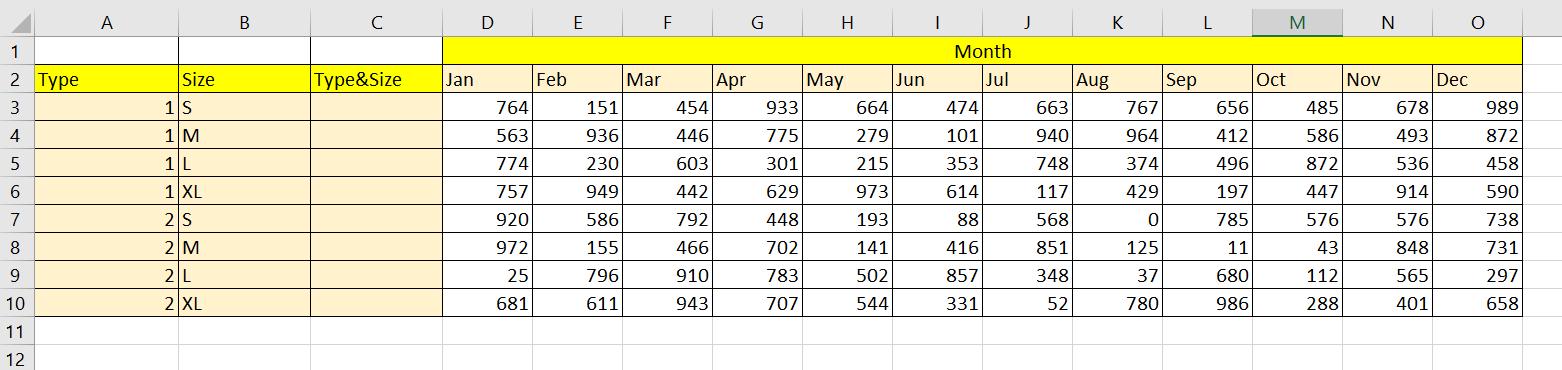
Suppose you have monthly sales data for a particular shirt. We have monthly data from January to December. Your stock includes two shirt designs in various sizes. To create a 3D table using month, size, and type as criteria, we can format the table like this:

Notice how we have several rows that correspond to each type-size combination. This allows us to represent three dimensions with a 2D array. 

We can use the INDEX and MATCH functions to find the sales figures of various criteria. The INDEX function allows us to find data in a 2D table when given a row number and column number. We can use the MATCH function to find the appropriate row and column number given a string to match.

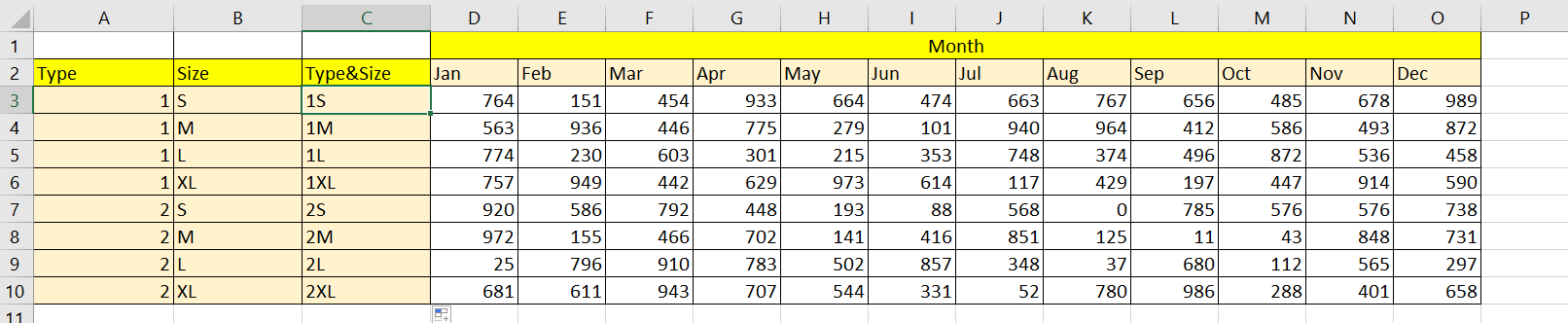
Since this method requires a single row input, we will have to create a new string out of the type and size criteria. We can simply combine type and size into a single criteria by using concatenation.

Now that we know what is needed to set up a 3D lookup table, let’s look into a few examples of 3D lookup tables in Microsoft Excel.

A Real Example of 3D Lookup Tables in Excel

Let’s take a look at a real example of a 3D lookup table on an Excel spreadsheet.

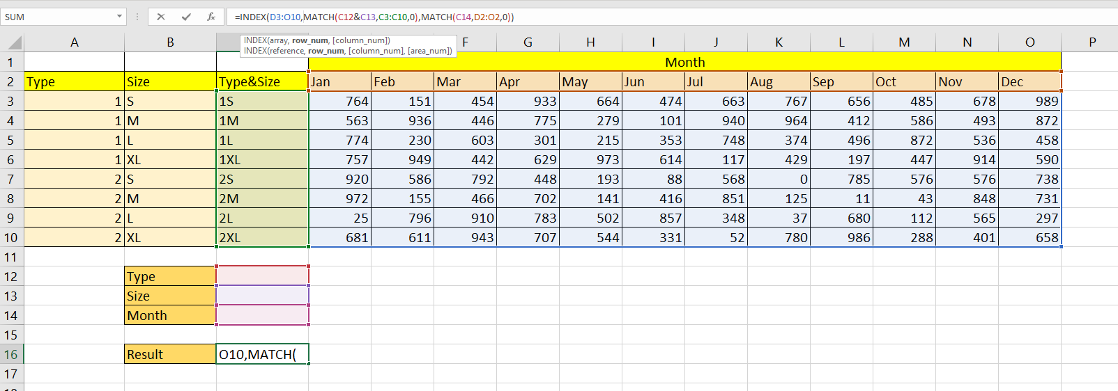
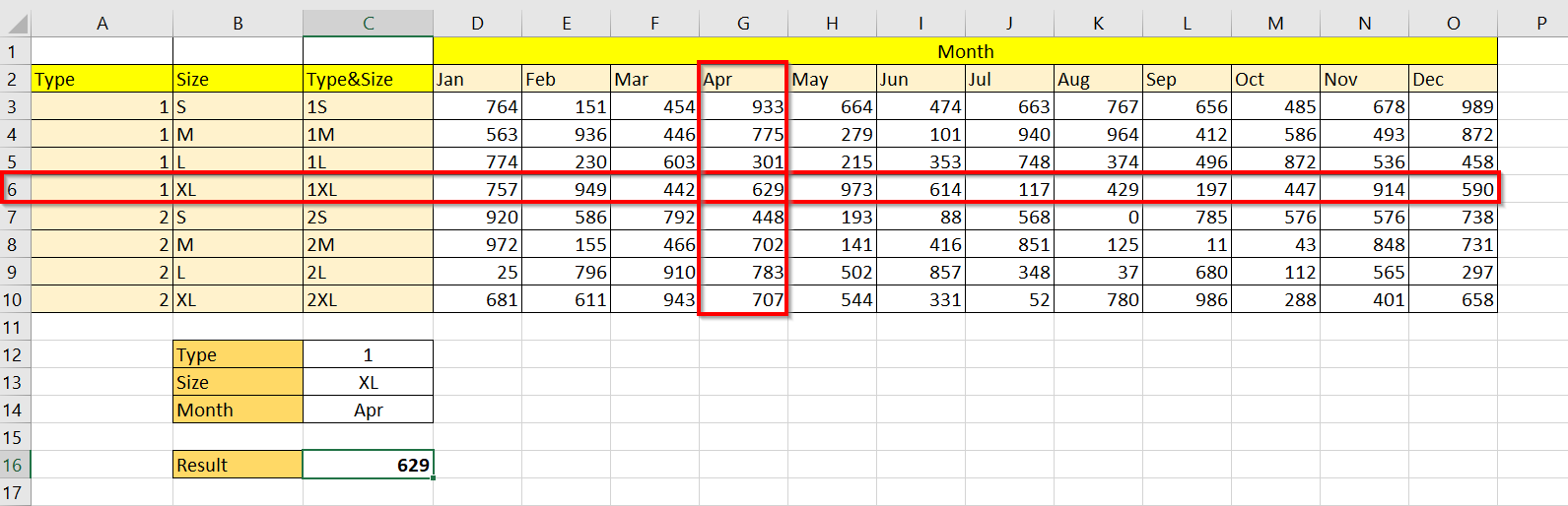
In the example below, we have three input criteria: type, size, and month. Users can input the appropriate values in cells C12, C13, and C14 to search through the lookup table. The answer, if found, will be displayed in cell C16.

To get the value in cell C16, we just need to use the following formula:

=INDEX(D3:O10,MATCH(C12&C13,C3:C10,0),MATCH(C14,D2:O2,0))

The formula uses an INDEX formula to return the value found in a table given a row number and column number. The first argument requires us to define the lookup table. In this example, our sales figures are in the cell range D3:O10.

Next, we must provide the row number for the second argument. We use the MATCH function to find the right type-size combination in the range C3:C10. For the final argument, we’ll use MATCH again to look for the specified month in the range D2:O2.

You can make your own copy of the spreadsheet above using the link attached below. 

If you’re ready to create your own 3D lookup table in Excel, let’s begin writing it ourselves. Follow the guide in the next section to learn how!

How to Lookup a Value in a 3D Table in Excel 

This section will guide you through each step needed to look up a value in 3D tables in Excel. You’ll learn how to use the INDEX and MATCH functions together to create a flexible lookup formula that allows you to input three criteria to search for.

This example will use the same T-shirt sales data seen in the previous sections. Our goal is to create a lookup table that allows the user to determine how many T-shirts are of a particular size and shape in a given month.

1. First, you must convert your three-dimensional data into a 2D table. In the example below, we’ve chosen to set up each row as a type/size pairing while each column corresponds to a specific month.
   
   
2. Next, we will add a new column after column B labeled ‘Type&Size’. This helper column will make finding the right row number easier later.
   
   
3. Use the formula =A3&B3 to concatenate the values in columns A and B. Fill the rest of the column with the same formula by dragging the cell down.
   
   
4. Next, add the INDEX and MATCH formula to the cell to display your result. The actual formula used will depend on the number of rows and columns your lookup table has. In the example below, we also added specific ranges to place user input.
   
   
5. Hit the Enter key to evaluate the function. Users can now input multiple criteria into the indicated cells to return the corresponding value in the lookup table.
   

Frequently Asked Questions (FAQ)

1. Why does my formula return an error?
   If your formula returns a #N/A error, then the lookup value cannot be found. You can use an IFERROR or IFNA function to catch this error if needed. If your formula returns a #REF! error, then your row and column values may point to a cell outside the specified array.

That’s all you need to remember to create your own 3D lookup table in Excel. This step-by-step guide shows how to use the INDEX and MATCH functions to look up values given three inputs.

Creating lookup tables is just one way users can take advantage of Excel functions. With so many other Excel functions out there, you can surely find one that suits your use case. 

Are you interested in learning more about what Excel can do? 

Make sure to subscribe to our newsletter to be the first to know about the latest guides and tutorials from us.

Get emails from us about Excel.

Our goal this year is to create lots of rich, bite-sized tutorials for Excel users like you. If you liked this one, you'd love what we are working on! Readers receive ✨ early access ✨ to new content.

Subscribe