This guide will explain how to add percentages to a pie chart in Microsoft Excel.
Table of Contents
Pie charts are an effective way to present data with multiple categories. This type of chart allows users to quickly determine the proportion of each category and its contribution to the total.
With Microsoft Excel, users can convert a dataset into a pie chart in just a few clicks. Excel also offers a range of customization options such as changing the color scheme, adding data labels, and adding legends. One of these options is adding percentages to the pie chart to enable users to clearly understand the size of each pie chart slice.
In this guide, we will provide a step-by-step tutorial on how to customize a pie chart with data labels showing percentage values.
A Real Example of Percentages in a Pie Chart in Microsoft Excel
Let’s explore a simple example where we can create a pie chart with percentages in Excel.
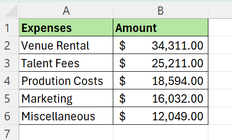
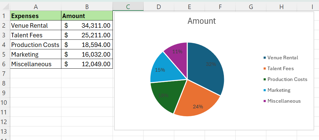
In the table above, we have a table containing a breakdown of expenses for a local music festival. We want to generate a pie chart to show how much each category contributes to the overall expense total.
We can select our data range and click Insert > Insert Pie or Donut Chart to add a new pie chart to our spreadsheet.
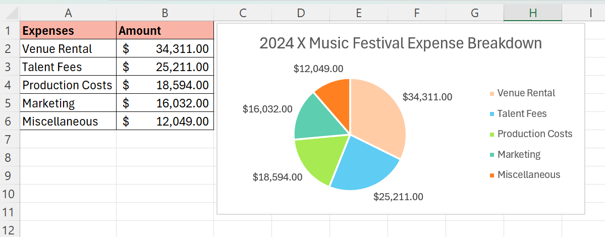
One issue we have with the generated chart above is that it can be difficult to determine the actual contribution of each category.
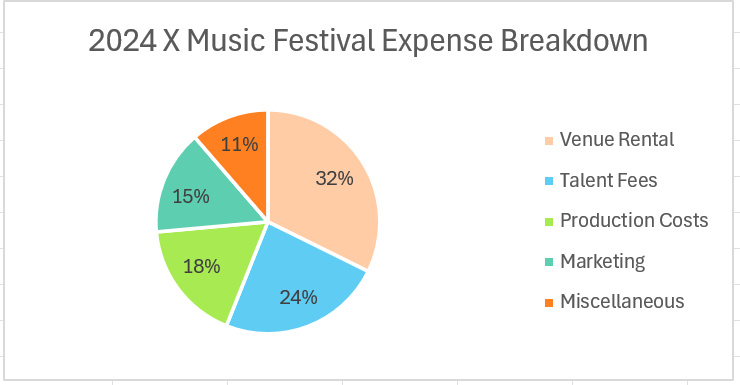
Excel allows users to customize a pie chart to show the percentage of each value instead of the absolute amount spent. For example, we can now read the chart above and see that we spent about 15% of our total expenses on marketing.
Click on the link below to create your own copy of our examples.
Head to the next section to read our step-by-step tutorial on how to add percentage values to your Excel pie charts.
How to Add Percentages to Pie Chart in Microsoft Excel
- First, select the data range to use for your pie chart.
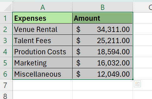
In this example, we’ll select the data range A2:B6 containing the dollar value in expenses of various categories for a local music festival. - Head to the Insert tab and click on the Pie chart icon under the Charts group.
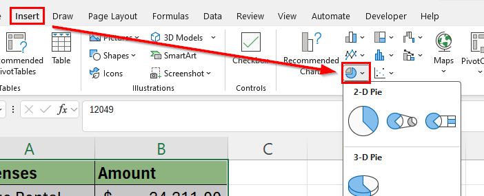
For this example, we’ll select the first 2-D pie chart type in the dropdown menu. - You should now see a pie chart in your sheet. The chart should be generated from the selected data range. In some cases, you may need to adjust the series to use if multiple series are provided in the data source.
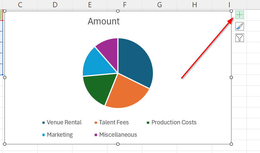
Select the pie chart and click on the Chart Elements option on the upper-right corner. This icon resembles a plus sign.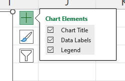
Next, ensure that the Data labels option is checked.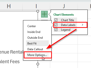
Click on the arrow to the right of Data Labels to reveal an additional menu. Click More Options.
- In the Format Data Labels panel, click on the checkbox of the Percentage option under Label Options > Label Contains.
- The pie chart should now have percentages added as data labels for each pie chart slice.
- Another way to display percentages is by clicking the Data Callout option under Data Labels.
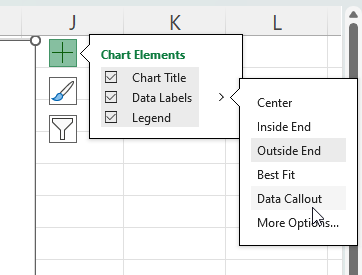
Data callouts are a more readable alternative to display percentages by showing data labels outside the slice in a text bubble shape.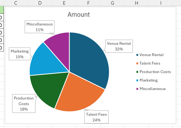
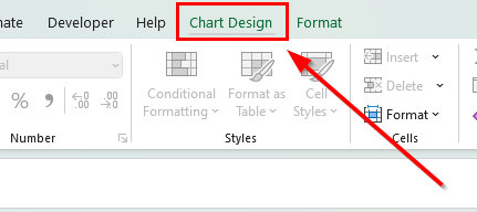
- We can also quickly add percentages to a newly-added pie chart by using the Quick Layout tool. First, click on your pie chart and select the Chart Design tab.
Click on the Quick Layout option and select any option with a percentage symbol.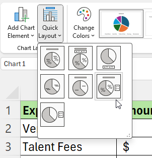
Excel will automatically reformat our chart to include data labels showing the percentage represented by each slice.
FAQs
- Can I display both values and percentages in a pie chart?
Yes, you can display both values and percentages in a pie chart. In the Format Data Labels pane, check both the Value and Percentage boxes. This will display both values and percentages on your chart. - How can I change the number of decimal places for the percentages?
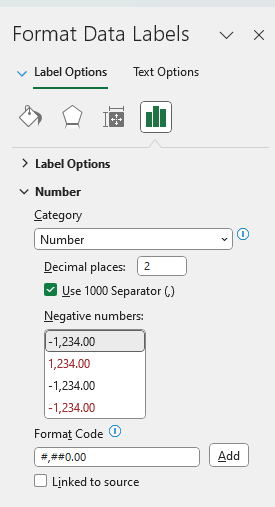
To change the number of decimal places for the percentages, go to the Format Data Labels pane and click the Number section. Choose Number or Percentage and set the number of decimal places you want.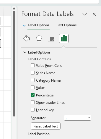
- Are the percentages updated automatically when my data changes?
Percentage data labels in your pie charts will update automatically when your data changes as long as your pie chart is linked to the data range.
To learn more about using charts and graphs in Microsoft Excel, you can read our post on how to create a gauge chart in Excel.
That’s all for this guide! Don’t forget to check out our library of spreadsheet resources, tips, and tricks for both Google Sheets and Microsoft Excel!