How to Use SUBTOTAL with AVERAGEIF in Excel

This guide will explain how to use SUBTOTAL with AVERAGEIF in Excel. 

The rules for using the SUBTOTAL function in Excel are the following:

• The nested subtotals are ignored to avoid double counting when there are other subtotals within ref1, ref2, or nested subtotals.
• The function will ignore any rows that are not included in the result of a filter no matter which function_num we use.
• The SUBTOTAL function does not support rows of data or horizontal ranges. 
• When any of the references are 3-D references, the function returns the #VALUE! error.

Excel is an excellent tool for organizing and calculating data. Whenever we have a large data set of values we need to calculate the total sum or average, the process is easier to perform in Excel due to built-in functions and tools.

But, sometimes we need to calculate only certain data in a large data set. So this is where we use the filter tool in Excel to only display the data values we need from the larger data set.

Usually, we would use the AVERAGEIF function to calculate the average of the data values. However, we get the total sum or average of the entire data set rather than just the filtered data values. 

Because the function calculates all the data values from the original data set, we can’t get the correct result from the filtered data. So we need another formula to use with the AVERAGEIF function to calculate what we need from the filtered data set correctly.

In this case, we can combine the SUBTOTAL function with the AVERAGEIF function to create a formula that will calculate the average of the filtered data set instead of the original data set.

Let’s take an example wherein we need to use SUBTOTAL with AVERAGEIF in Excel.

Suppose you have a master list of all your students’ scores from different classes. And you need to calculate the class average for each gender. Since you do not want to create a new table for each class, you opted to filter out the specific class you want to calculate the average. 

However, you cannot get the correct result since the function includes the data values from the original data set instead of just the filtered ones. Instead, you combine SUBTOTAL with AVERAGEIF to get the correct result.

Before we move on to a real example, let’s first learn the syntax of the two functions in Excel.

The Anatomy of the SUBTOTAL Function

The syntax or the way we write the SUBTOTAL function is as follows:

=SUBTOTAL(function_num, ref1)

Let’s take apart this formula and understand what each term means:

• = the equal sign is how we can activate any function in Excel.
• SUBTOTAL() refers to our SUBTOTAL function. This function is used to return the subtotal in a list or database.
• function_num is a required argument. And it refers to a number from 1 to 11 that will specify the summary function for the subtotal. 
• ref1 is another required argument. So it refers to 1 to 254 rangers or cell references for which we want to find the subtotal. 

The Anatomy of the AVERAGEIF Function

The syntax or the way we write the AVERAGEIF function is as follows:

=AVERAGEIF(range, criteria, [average_range])

Let’s take apart this formula and understand what each term means:

• = the equal sign is we begin any function in Excel.
• AVERAGEIF() is our AVERAGEIF function. So this function is used to find the average or arithmetic mean for the selected cells based on a given condition or criteria. 
• range is a required argument. And it refers to the range of cells we want to be evaluated.
• criteria is also a required argument. So it refers to the condition or criteria in the form of a number, expression, or text that defines which cells we want to use to find the average.
• average_range is an optional argument. And it refers to the actual cells to be used to find the average. If left blank, the cells in the range are used. 

Great! Now let’s discuss a real example of using SUBTOTAL with AVERAGEIF in Excel.

A Real Example of Using SUBTOTAL with AVERAGEIF in Excel

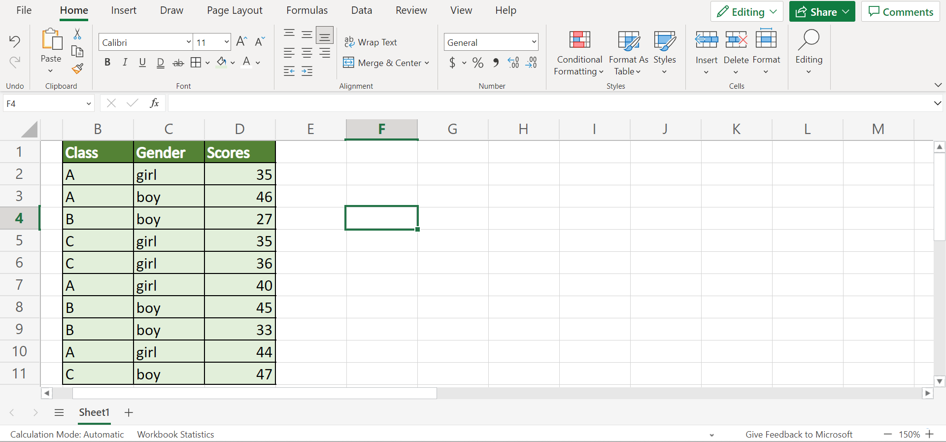
Let’s say we have a data set containing a list of the class section, the gender of the student, and their scores. And we want to calculate the average of the girls’ scores in a specific class. So our initial data set would look like this:

Firstly, we need to filter our original data set. Since we only want to calculate the average of a specific class, we will filter the data set only to show that specific class. 

Once we have filtered out the data set, we are left with the specific class we want to calculate the average of. In this case, we want to focus on the average score of the girls in this class. 

If we only use the AVERAGIF function alone, the function will calculate all the girls’ scores, including those from the other classes. To prevent this, we will combine the AVERAGEIF function with the SUBTOTAL function to correctly calculate only the filtered values. 

And our final data set would look like this:

You can make your own copy of the spreadsheet above using the link attached below. 

Amazing! Now we can explain the steps of how to use SUBTOTAL with AVERAGEIF in Excel.

How to Use SUBTOTAL with AVERAGEIF in Excel

In this section, we will explain the step-by-step process of how to use SUBTOTAL with AVERAGEIF in Excel. Furthermore, each step contains pictures and detailed instructions to guide you along the way. 

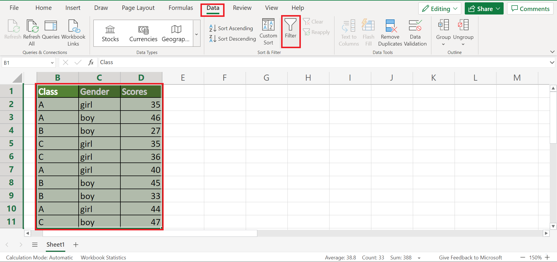
1. Firstly, we need to filter our data set. In this case, we only want to display the values from class A. To do this, we will first select the entire data set and go to the Data tab. Then, we will click the Filter icon.

2. Secondly, we will click the dropdown arrow beside the Class column. Next, we will check the box beside A to only display those data values. Then, we will click Apply.

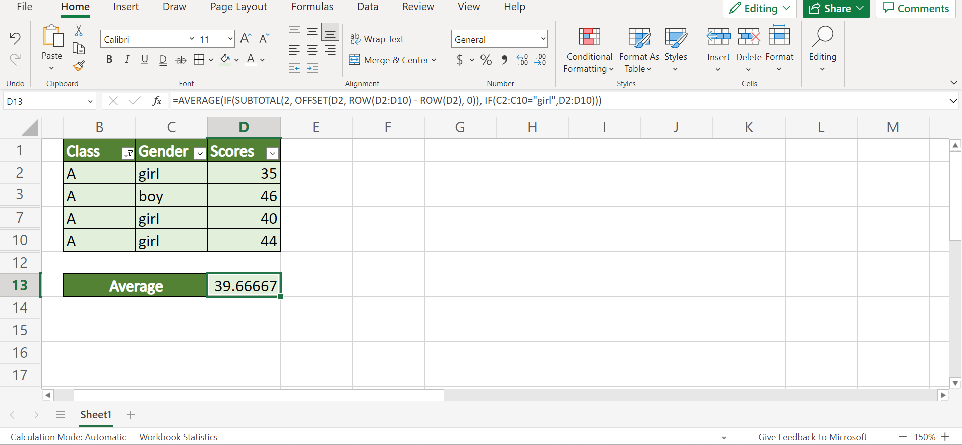
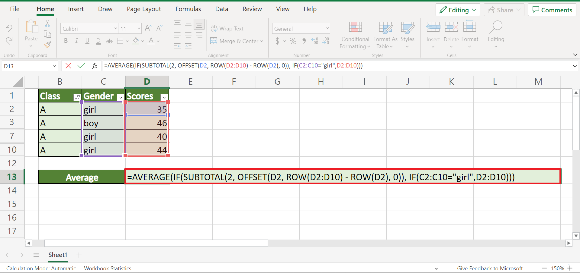
3. Thirdly, we can now use a combined SUBTOTAL and AVERAGEIF formula to calculate the average of the filtered data values. So we will type in the formula “=AVERAGE(IF(SUBTOTAL(2, OFFSET(D2, ROW(D2:D10) – ROW(D2), 0)), IF(C2:C10=”girl”,D2:D10)))”.

Lastly, we will press the Enter key to return the result.

4. And tada! We have correctly calculated the average of the filtered data values.

And that’s pretty much it! We have explained how to use SUBTOTAL with AVERAGEIF in Excel. Now you can apply this learning whenever you need to calculate the average values of a filtered data set.

Are you interested in learning more about what Excel can do? You can now use the SUBTOTAL function and the various other Microsoft Excel formulas available to create great worksheets that work for you. Make sure to subscribe to our newsletter to be the first to know about the latest guides and tutorials from us.

Get emails from us about Google Sheets.

Our goal this year is to create lots of rich, bite-sized tutorials for Google Sheets users like you. If you liked this one, you'll love what we are working on! Readers receive ✨ early access ✨ to new content.

Subscribe