This guide will discuss how to use DATETIME criteria within the FILTER function in Google Sheets.
A DATETIME criterion, which is essentially a timestamp within the FILTER function does not perform appropriately in Google Sheets. So we need to use additional functions to help us perform this task.
Although we can FILTER by date and time separately, there will be times you are required to FILTER both date and time together.
FILTER function filters data from a specified range based on the given criterion. And FILTER does not support conditions for both columns and rows. It can only be either specified columns or rows.
A DATETIME criterion is a value that contains both a date and a time. Also, the date and time format must be consistent when using the FILTER function to get the correct results.
Since it is a DATETIME criterion, you cannot simply use the FILTER function. You can use the ISBETWEEN function or comparison operators in the FILTER formula to filter the data correctly.
The ISBETWEEN function is useful in determining if a value is within a specific range or not. While comparison operators are used in comparing and evaluating numbers. The operators are less than (<), greater than (>), equal to (=), less than or equal to (<=), greater than or equal to (>=), and not equal to (<>).
Let’s take a scenario.
Suppose you want to filter the names of those who submitted the survey within the deadline. You opened the survey on 3/13/2002 at 10:00 AM.
So your condition would be those who submitted on or before 3/15/2022 at 11:30 AM. Then, you used the ISBETWEEN function within the DATETIME criteria to filter the specific names.
Great! Let’s dive into a real example of how to use DATETIME criteria within the FILTER function in Google Sheets.
A Real Example of How to Use DATETIME Criteria within FILTER Function in Google Sheets
First, let’s look into a sample dataset that we will use to filter based on a DATETIME criterion. We have a dataset containing each employee’s clock-in and clock-out times in one day.
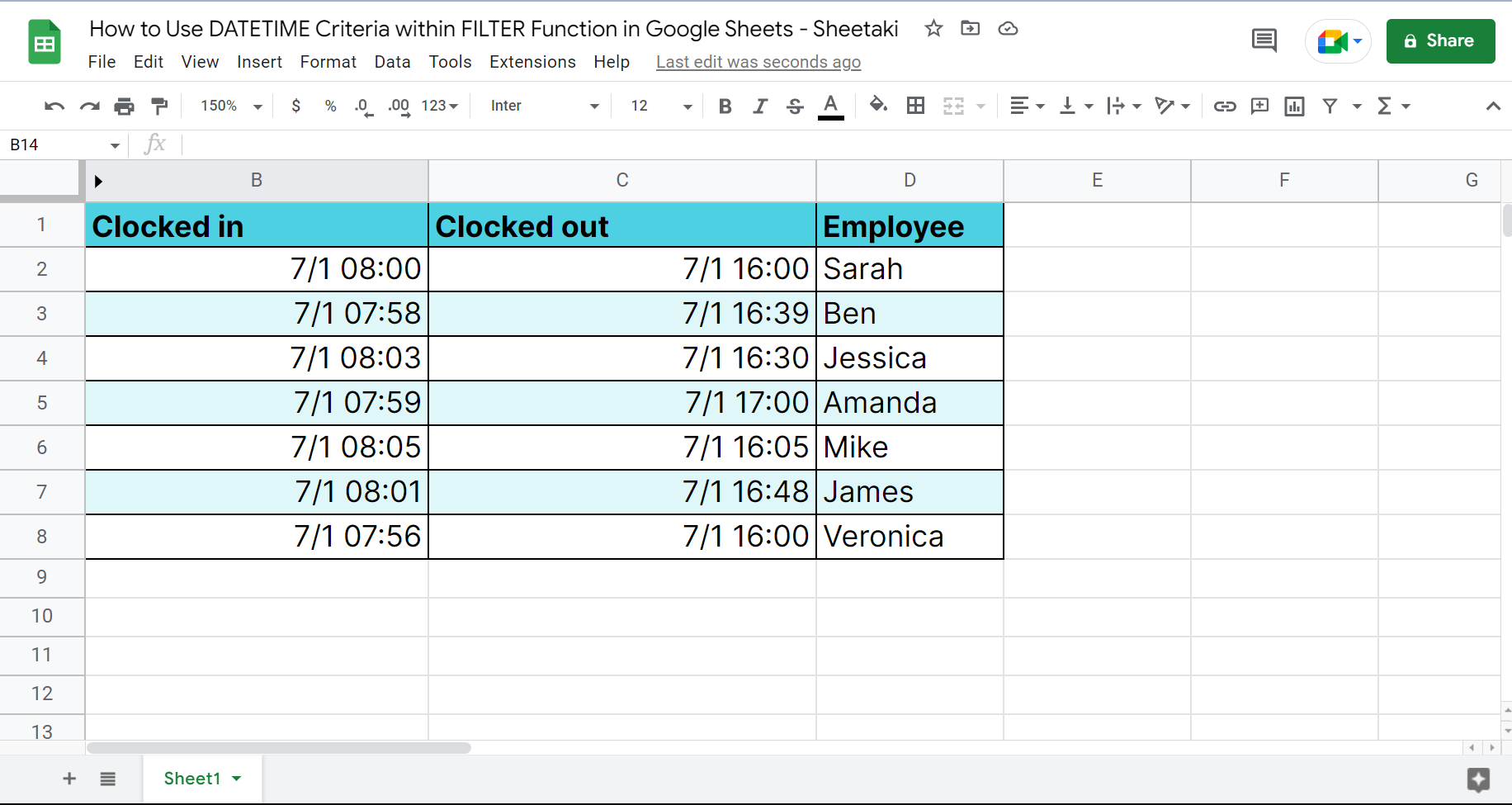
For instance, we want to filter out the employee who did overtime for that day. So the office hours would be from 8:00 AM to 4:00 PM. And overtime hours are from 4:01 PM to 6:00 PM.
But, we need to format the date and time first. In this case, we will follow the Day/Month/Year Hour:Minute:Second format. Then, we can use the FILTER function to filter employees who clocked out between 4:01 PM and 6:00 PM.
Finally, this is what the final output would look like after using the DATETIME criteria within the FILTER function in Google Sheets.

So Ben, Jessica, Amanda, Mike, and James are the employees who did overtime on 7/1/2022.
You can make your own copy of the spreadsheet above using the link attached below.
Now let’s move on from this example. And let’s learn the process of how to use DATETIME criteria within the FILTER function to apply to our work.
How to Use DATETIME Criteria within FILTER Function in Google Sheets
This section will explain the steps on how to use DATETIME criteria within the FILTER function in Google Sheets in two ways: the ISBETWEEN function and comparison operators.
1. First, prepare the dataset by formatting the date and time. To do this, go to Format. Then, click on Number. From the dropdown menu, click Custom date and time.

2. Second, input the desired format of the date and time. In this case, we will follow the format Day/Month/Year Hour:Minute:Second.

If this format is unavailable on the list, you can click on the drop-down arrow at the top right of the search bar. From here, you can select the format you want. Then, click Apply.
3. Furthermore, we can check if the date format is correct using the DAY function. Simply click on any blank cell. Input the DAY function and select any date from the dataset to check. If the returned number is the day of the month, the date format is correct.
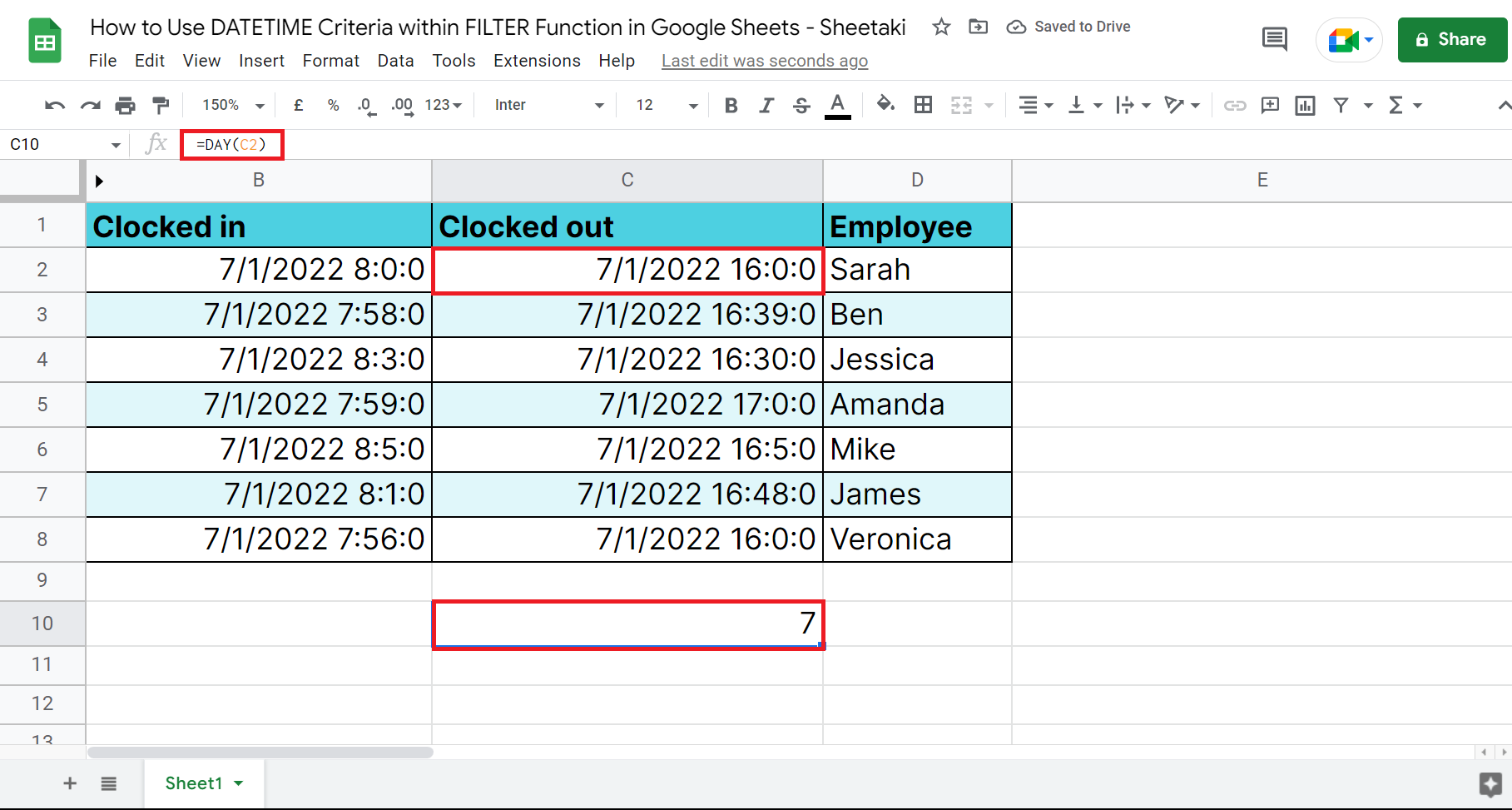
In this case, we checked the date on C2. Since the date is 7/1/2022, the returned value must be 7.
4. Create a separate table where you want to place the filtered data. In this case, we will input the formula on F2. First, let’s try this formula ‘=FILTER(C2:D,ISBETWEEN(C2:C,DATE(2022,1,7)+TIME(16,1,0),DATE(2022,1,7)+TIME(18,0,0), FALSE,FALSE))’.

This method uses the ISBETWEEN function with the FILTER function to successfully filter DATETIME criteria. Since we want to filter out the employees based on their clocked-out time, the range would be C2:D.
And the ISBETWEEN is used to formulate the DATETIME criteria of the overtime hours, which are between 4:01 PM and 6:00 PM on the date 7/1/2022.
5. If the first method did not work for you, you can also use comparison operators. In this case, input the formula ‘=FILTER(C2:D,C2:C>DATE(2022,1,7)+TIME(16,0,0),C2:C

We still have the same criteria but just a different way of expressing it. This time we expressed the overtime criteria as greater than (>) 7/1/2022 4:00 PM and less than (<) 7/1/2022 6:00 PM.
6. And tada! We have successfully filtered out the employees who did overtime on 7/1/2022.
Amazing! You have learned how to successfully use DATETIME criteria within the FILTER function in Google Sheets to filter out data that contain both date and time. Now you can efficiently deal with DATETIME criteria when using the FILTER function.
Are you interested in learning more about what Google Sheets can do? You can now use the FILTER function in Google Sheets and the various other Google Sheets formulas available to create great worksheets that work for you. Make sure to subscribe to our newsletter to be the first to know about the latest guides and tutorials from us.