How to Alphabetize and Keep Rows Together in Google Sheets

Google Sheets has built-in sorting functions that are useful when you need to alphabetize your dataset.

There are multiple ways to sort your data. The SORT function allows you to alphabetize a selected range of data, a column, or multiple columns. We can also take advantage of the built-in sort options. 

Let’s look at a scenario where we might need to alphabetize our data.

You have a spreadsheet of participants that you want to interview. Your team has decided to interview them in alphabetical order according to their last name. What’s the best way to sort the participant data to create a tracker?

Google Sheets comes with a built-in sort feature that can easily sort your spreadsheet in a few clicks. The problem, however, is that adding new participants does not automatically re-sort our tracker.

Luckily, we have another way to alphabetize our data. With the SORT function, we can quickly sort our dataset dynamically.

Let’s learn how to alphabetize our data ourselves in Google Sheets and later test it out using an actual dataset.

Using the Built-In Sort to Alphabetize in Google Sheets

Let’s look at a real example of alphabetizing rows in a Google Sheets spreadsheet.

In the example below, we’ve sorted a dataset of employees by their last name in alphabetical order. 

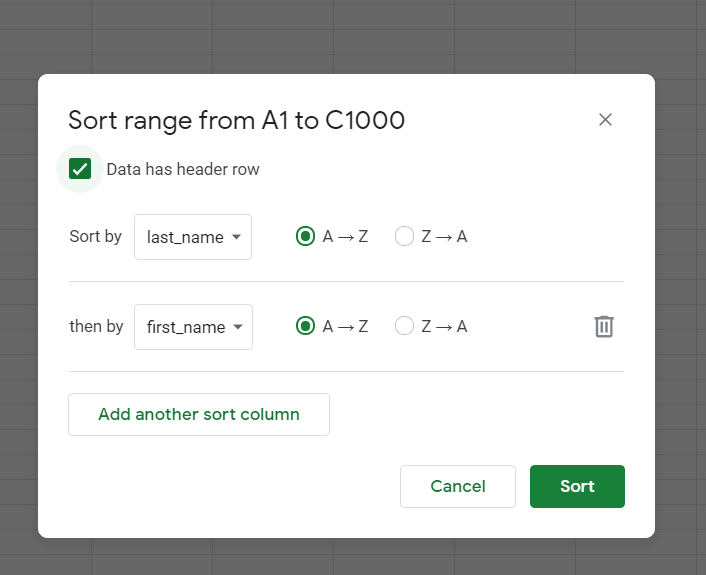
To get these values, we had to use the built-in Sort range feature in Google Sheets. By default, this feature sorts a range by the first column. Since we needed to sort by the second column, we used advanced range sorting options.

We may also set multiple columns as sort columns. For example, we could sort our elements by the last name, and if any participants share the same last name, they’d be sorted by their first name.

This type of sorting is static rather than dynamic. This means that once we do the sort once, it won’t automatically sort the dataset if we add or change any values in our dataset. 

In the next section, we’ll explore a more dynamic way of alphabetizing our datasets.

Using SORT Function in Google Sheets

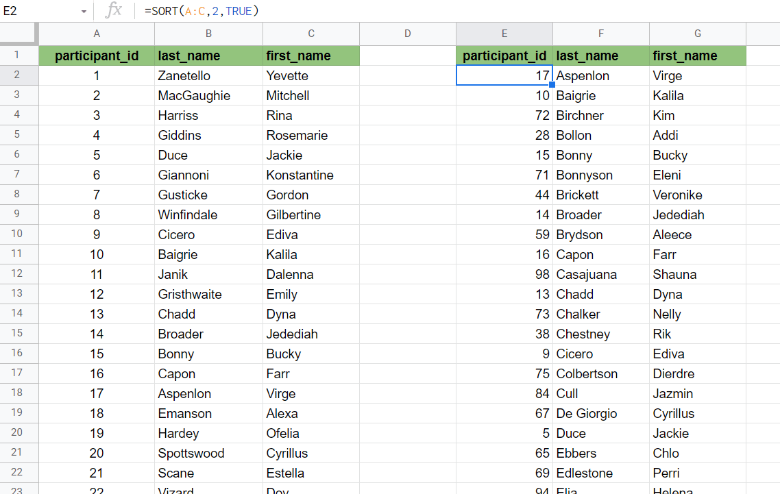
In the example below, we alphabetized the range A2:C101 by the last name using the SORT function. You can confirm this by looking at the values seen in column F.

To get the values in the second table, we just need to use the following formula in cell E2:

=SORT(A2:C,2,TRUE)

The first argument indicates the range to sort. The second argument refers to the column to alphabetize by, which in this example is the 2nd column in the range. Finally, the third argument tells us whether to sort it in ascending order.

In the example below, we set the last argument to FALSE. This sorts the dataset in reverse alphabetical order.

Using the SORT function is a dynamic way of sorting data. This means that if we make any changes or additions to the original range, the output of SORT will update as well.

You can make your own copy of the spreadsheet above using the link attached below. 

If you’re ready to try out these sorting methods in Google Sheets, let’s start writing them ourselves!

Keeping Rows Together in Google Sheets

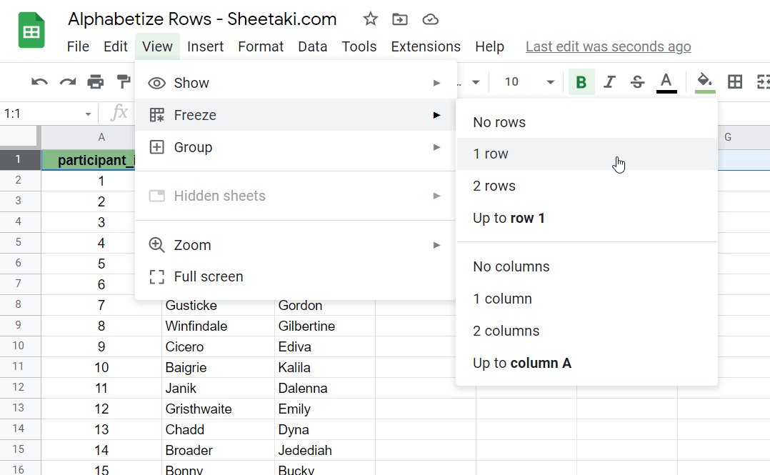
When sorting, you might become frustrated if your table headers are sorted as well. To prevent this from happening, we can use the Freeze option to lock the rows in place.

In the table below, we have frozen the first row. Now, when we use the built-in sorting options, the first row will be excluded from the sorting.

How to Alphabetize and Keep Rows Together in Google Sheets

In this section, we will go through each step needed to start alphabetizing and keeping rows together in Google Sheets.

Follow these steps to start using alphabetizing your dataset:

1. First, we’ll demonstrate sorting the dataset with the SORT function. We’ll copy the column headers and begin with the leftmost column in this range.
   
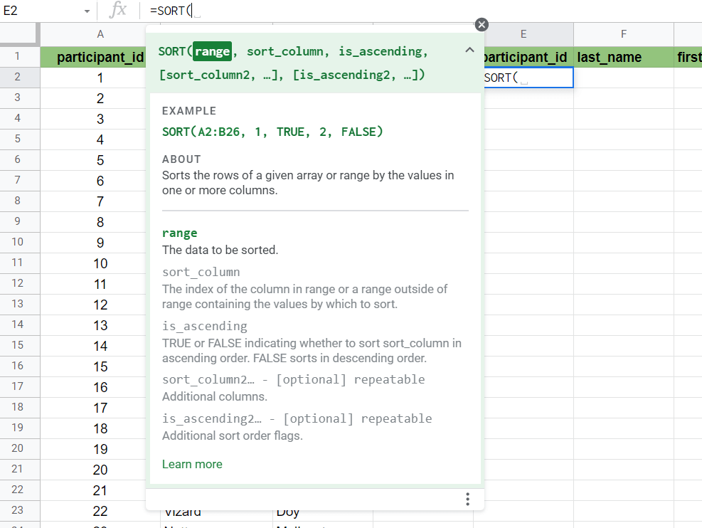
2. Next, we simply type the equal sign ‘=‘ to begin the function, followed by ‘SORT(‘. 
3. You might encounter a pop-up with hints on how to use the SORT function. Clicking on the arrow in the top-right-hand corner of the pop-up will minimize it.
   
4. Next, we’ll have to fill in the arguments for this function. This is simply the range to sort, which column to sort by, and whether to sort it in ascending order.
   
5. In these last couple of steps, we’ll show you how to use the built-in sort feature. First, we’ll have to freeze the first row. You can find the Freeze option under the View menu.
   
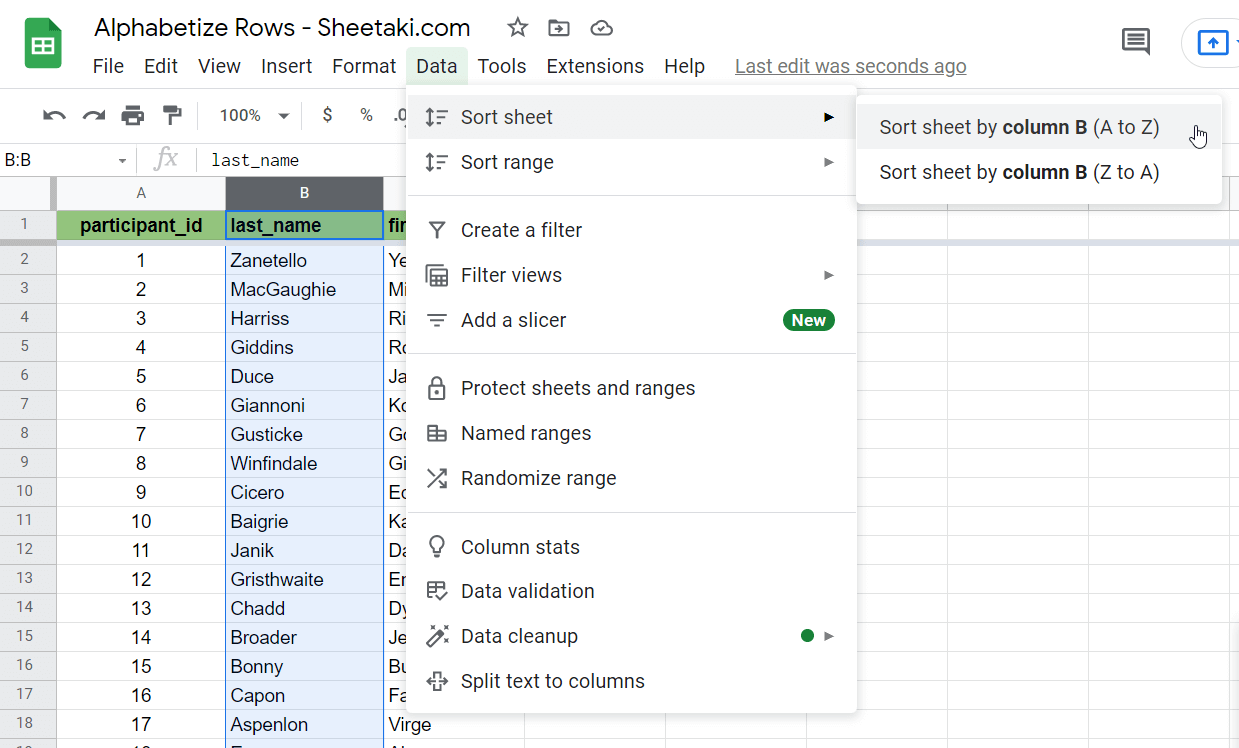
6. Next, select the column that we’ll be sorting by. In this example, we’ll again sort by last name.
   
7. Since we’ve already frozen the first column, we can sort the entire sheet. We can find this option under the Data menu. We’ll sort the sheet in alphabetical order (A to Z). 
   
8. As seen below, we kept the first row at the top while having the rest of our dataset alphabetized by the last name.
   
   

That’s all you need to remember to alphabetize and keep rows together in Google Sheets. This step-by-step tutorial shows how simple it is to sort methods in both static and dynamic.

Sorting your dataset is just one example of what you can do with your data in Google Sheets. With so many other Google Sheets functions out there, you can indeed find one that best fits your needs.

Are you interested in learning more about what Google Sheets can do? Make sure to subscribe to our newsletter to be the first to know about the latest guides and tutorials from us.

Get emails from us about Google Sheets.

Our goal this year is to create lots of rich, bite-sized tutorials for Google Sheets users like you. If you liked this one, you'd love what we are working on! Readers receive ✨ early access ✨ to new content.

Subscribe