How to Use OR Function in Google Sheets

The OR Function in Google Sheets is useful if you want to check whether or not your data range is TRUE or FALSE.

The OR function does this simply by using it together with logical expressions in your Google Sheets.

It is a stand-alone function. Meaning, it can stand on its own. You can use it as it is. But, most often, it is paired with other functions such as, but not limited to IF.

The use of the OR function makes sense especially if you are working on large data and you want to check if your logical expressions are TRUE or FALSE. After you supplied the logical expressions, the OR function will then see if one of the expressions is TRUE. If it is, then it returns TRUE. At this point, you might be wondering, what is a ‘logical expression’. As we go on with this guide, we will learn the terminologies, what it is, and how to work with the OR function in Google Sheets.

Working with the OR function is easy because even if you have a lot of logical expressions contained in your formula, it will just see if there’s at least one expression that’s TRUE. The formula will only return a TRUE or FALSE answer.

Let’s take an example to understand this concept better.

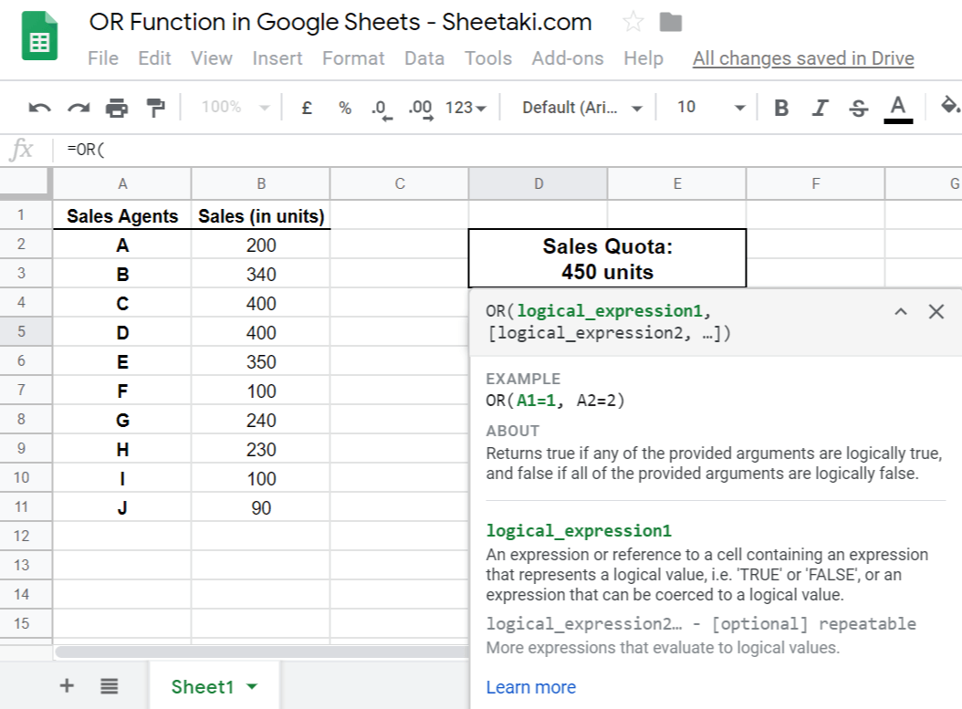
Say you are a sales manager that has 20 sales agents. You want to check if there’s even one who reached the sales quota. Instead of checking their sale one by one, you can simply use the OR function to make the work faster. Let’s say your sales quota is 450 units. Using the OR function, you can take your agents’ sales and use a comparison operation, which is, in this case, an equal sign ~ equal to 450 units.

After you hit on the ‘Enter’ key, it will then give you a TRUE or FALSE answer. Remember, the OR function will only see if there’s at least 1 TRUE expression. Even if you drag down the formula, it will still give you the same output.

Easy, right?

You’ll better appreciate the OR function if you nest it with other functions, most especially the IF function.

The Anatomy of the OR Function

So the syntax (or the way we write) the OR function is as follows:

Here’s how it will look like:

=OR(logical_expression1, [logical_expression2, ...])

Let’s break this down to better understand what each term means:

• = every function in the Google Sheet starts with an equal sign.
• OR() this is our function. We need to add attributes for it to work properly in Google Sheets.
• logical_expression1 is a required attribute as this refers to the condition that is being tested. Normally, we use comparison operators > (greater than), < (less than), and = (equal), to help form the condition (eg. A2 > 60 ~ The cell A2 is greater than 60.) You can also use both if need be.
• logical_expression2, logical_expression3 and subsequent logical expressions are optional additional conditions which you may add should you need to evaluate them. There is no limit to how many logical_expressions you can add.

It may look too easy or a bit hard to understand, but we assure you that towards the end, you will surely feel comfortable applying the OR function in Google Sheets. So hang in there! 🙂

A Real Example of Using OR Function

Take a look at the example below to see how OR function is used in Google Sheets.

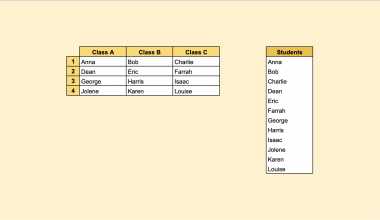
In the example above, we have 10 sales agents in the name of A, B, C, up to J. Each sales agent has his own sale in units. We want to check if there’s even one among sales agents A to E that has met the sales quota for a specific month.

Here’s what this example does:

• We have actively selected D5 and we want to use the OR function to check if there is any among the selected 10 agents, have met the 450-unit quota.
• Since we are checking the sales of agents A to E, we now know that we have 5 logical expressions to add.
• After identifying how many logical expressions should we have, we then created each of them.
• In this particular example, we want to check if there is one among sales agents A to E has reached the 450-unit quota. In that case, our expression is, greater or equal to 450. So, we used the >= sign.
• For the first logical expression, we had B2>=450. The second is B3>=450. And so on up to B6, the sale of agent E.
• We ended the formula with a close parenthesis, and we got the result, TRUE.

Easy, right?

You may make a copy of the spreadsheet using the link I have attached below:

Let’s begin writing our own OR function in Google Sheets.

How to Use OR Function in Google Sheets

I changed the data a bit to show you how it would look if none of the agents meet the 450-unit quota. The process is still the same. Let’s get to work!

1. Simply click on an empty cell to make it active. This is where we want to write our formula. For this guide, I will be selecting D5.

2. Next, simply type in an equal sign (=), followed by OR, which is our function. Since you’re beginning the function, do not forget to add the opening parenthesis ‘(‘.

3. Wait for the pop-up message as this will be your guide to writing the formula perfectly.

4. Now what you need to do is to carefully select the data that you want to check, followed by the comparison operators, >=, then the 450. We started off with the cell B2.

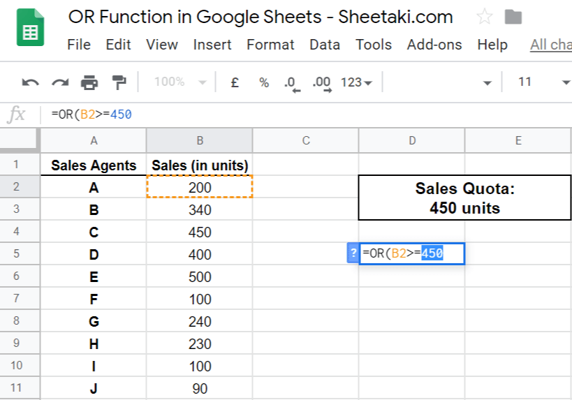
5. Continue the process until you reach the cell B6, each separated with a comma ‘,‘.

6. Close your formula with a close parenthesis ‘)‘ , then hit on the Enter key.

You may want to check the next 5 agents’ sales to see whether or not the answer is still TRUE.

That’s pretty much it. You can now use the OR function together with the other numerous Google Sheets formulas to create even more powerful formulas that can make your life much easier. 🙂

Get emails from us about Google Sheets.

Our goal this year is to create lots of rich, bite-sized tutorials for Google Sheets users like you. If you liked this one, you'll love what we are working on! Readers receive ✨ early access ✨ to new content.

Subscribe