


This guide will discuss how to calculate the cost of funds in Excel.
The cost of funds is most often used in banking, finance, and companies. And most companies will calculate their cost of funds to know how much they need to earn to keep the investment worthwhile.
Furthermore, financial institutions calculate the costs of funds to identify how much money they need to acquire funds to lend or loan to businesses.
So the cost of funds refers to the rate of interest financial institutions and banks pay on their debt or the money they borrowed to operate their business. Basically, it is an interest rate charged to obtain or get funds.
Essentially, the cost of funds is a total of all the blended costs of all sources of funds. And the formula for the costs of funds is the weighted average cost of capital or WACC.
The weighted average cost of capital is obtained by multiplying the proportion of each fund source by its price and adding the results.
Let’s take a scenario.
Suppose you are an employee in a financial institution. And you were tasked to calculate the cost of funds for the funds a certain company borrowed. Although you can calculate WACC manually, utilizing Excel to calculate it would be easier and have a lesser chance of error.
Great! Now let’s discuss a real example of calculating the cost of funds in Excel.
A Real Example of Calculating Cost of Funds in Excel
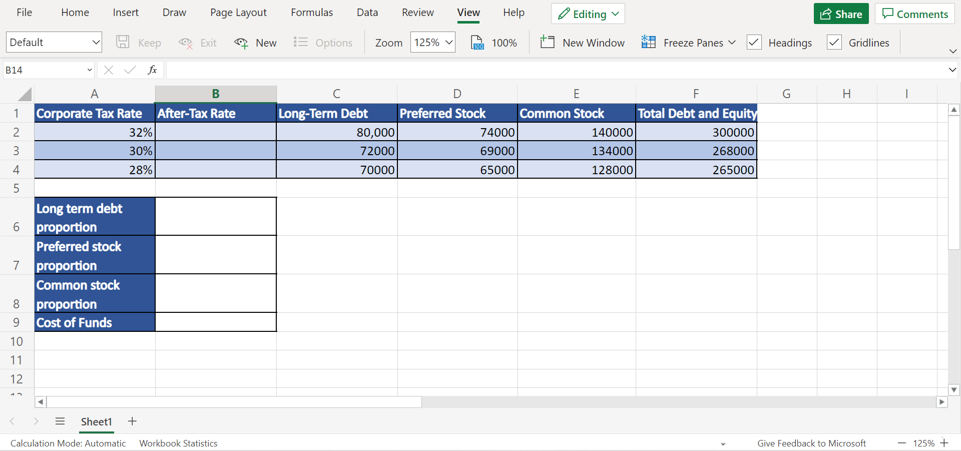
Firstly, we need to prepare our data set by inputting all the needed components to calculate the weighted average cost of capital or WACC. So this would be the corporate tax rate, long-term debt, preferred stock, common stock, and total debt and equity.
So the formula for calculating the WACC is the cost of funds = LTP + PSP + CSP. Whereas LTP refers to long-term debt proportion, PSP is the proportion of preferred stock, and CSP refers to the proportion of common stock.
Long-term debt is a liability of a company. And the preferred stock of a company refers to an aggregation of the aspects the common stock does not contain. Lastly, common stock refers to security, representing ownership in a company or corporation.
And this is what our Excel sheet would most likely look like once we input all the necessary components.
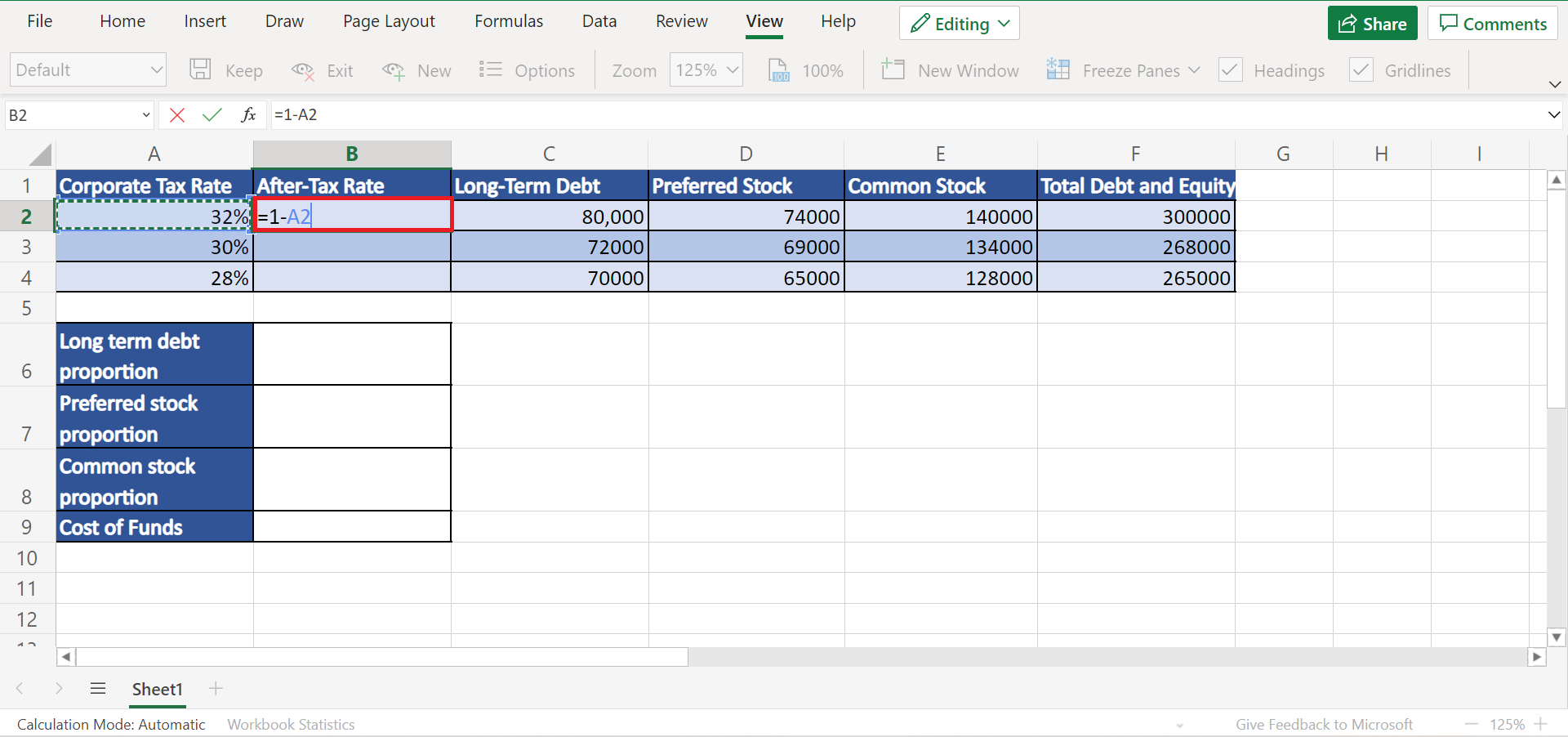
Secondly, we need to obtain the after-tax rate, which is done by the formula of =1 - corporate tax rate. Then, we will calculate the proportion of the long-term debt, preferred stock, and common stock. Lastly, we will calculate the cost of funds using the WACC formula.
And this is our final output.
You can make your own copy of the spreadsheet above using the link attached below.
Awesome! Let’s finally discuss the steps of how to calculate the cost of funds in Excel.
How to Calculate Cost of Funds in Excel
In this section, we will explain the step-by-step process of how to calculate the cost of funds in Excel.
1. Firstly, we need to prepare the data set. So we will create a table containing the necessary information we need. For instance, the corporate tax rate, after-tax rate, long-term debt, preferred stock, common stock, and total debt and equity.
Moreover, we will prepare a table below where we will input the WACC calculations. So this will contain the proportion of the long-term debt, preferred stock, and common stock. Lastly, it will have a row for the cost of funds result.
2. Secondly, we will calculate the after-tax rate. So input the formula =1 - corporate tax rate. In this case, our formula will be “= 1-A2”.
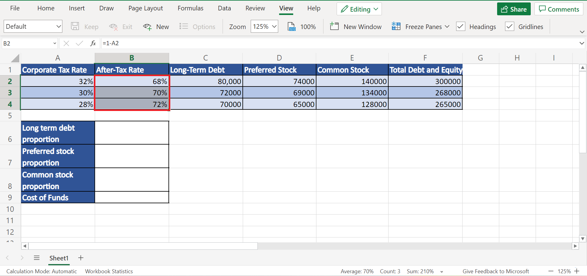
3. Thirdly, drag down to copy the formula to the rest of the after-tax rate rows.
4. Next, we will calculate the long-term debt proportion. For example, our interest rate would be 8%. To calculate the long-term debt proportion, input the formula “=(C2/F2)*B2*8%”.

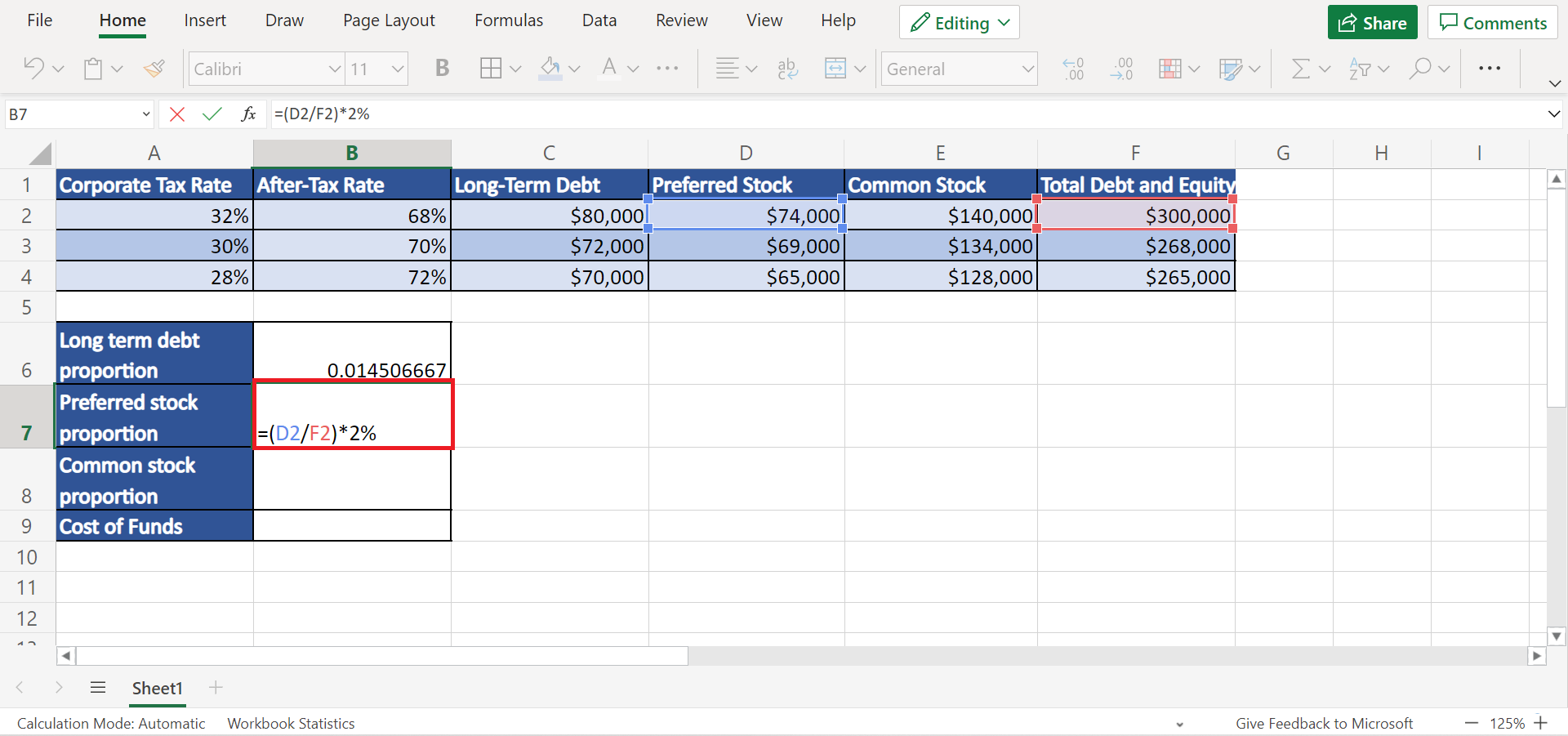
5. Then, it’s time to calculate the preferred stock proportion. In this case, let’s say our percentage rate for our preferred stock is 2%. So we will input the formula “=(D2/F2)*2%”.
6. Next, let’s calculate the common stock proportion. For instance, our minimum amount of profit return for our data set is 10%. To calculate the common stock proportion, input the formula “=(E2/F2)*10%”.

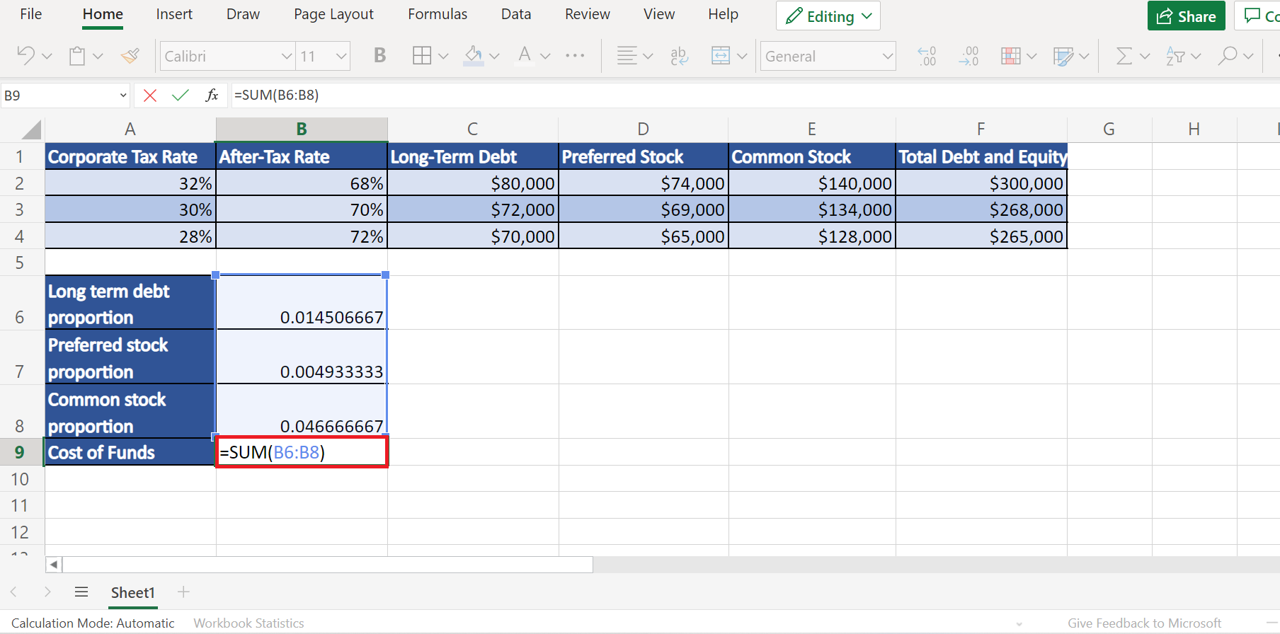
7. Finally, it’s time to calculate the cost of funds since we have obtained the proportions of all needed components. Firstly, we will add all the proportions. So type the formula “=SUM(B6:B8)”. And press the Enter key to return the result of the cost of funds.
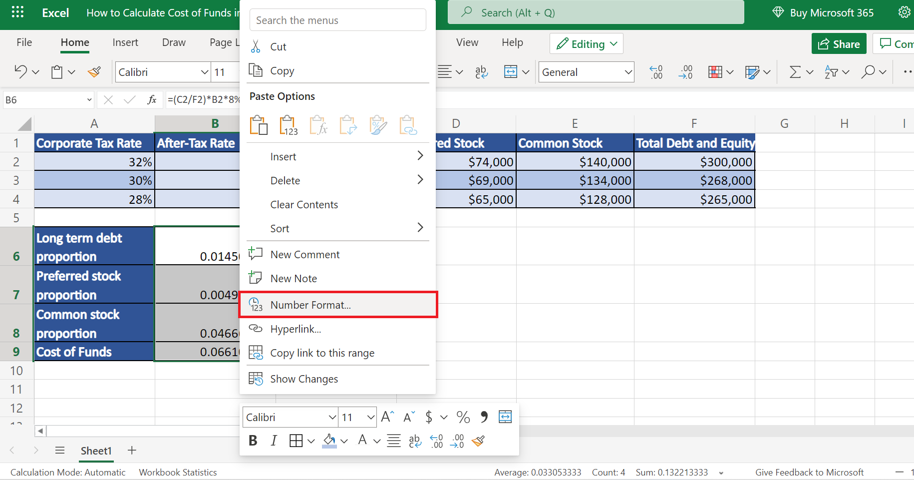
8. Additionally, let’s change the format of our results, so they return as percentages. Firstly, select the three components and right-click. Then, select Number Format.
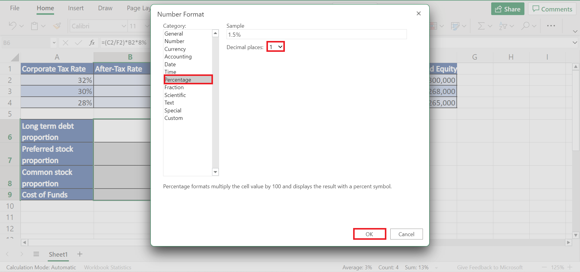
9. In the Number Format window, go to Percentage. And select 1 in the Decimal places. Lastly, click OK to apply changes.
10. And tada! We have successfully calculated the cost of funds in Excel.

That’s pretty much it! Wasn’t it quite easy and simple? Now you can calculate the cost of funds in Excel whenever you need to.
Are you interested in learning more about what Excel can do? You can now use the various other Microsoft Excel formulas available to create great worksheets that work for you. Make sure to subscribe to our newsletter to be the first to know about the latest guides and tutorials from us.


