This guide will explain how you can use the RANK function to rank a non-continuous range in Excel.
The RANK function allows you to give a numeric rank to a value in comparison to other values in the list. While users commonly rank values that belong to a single range, Excel gives us the option to rank non-continuous cells.
The rules for using the RANK function in Excel are as follows:
- The function requires three arguments: the number to rank, the list of values to rank against, and whether to rank in ascending or descending order.
- The function then outputs an integer that indicates the rank of the chosen value.
Let’s take a look at a quick example of when you might need to rank values in a non-continuous range in Excel.
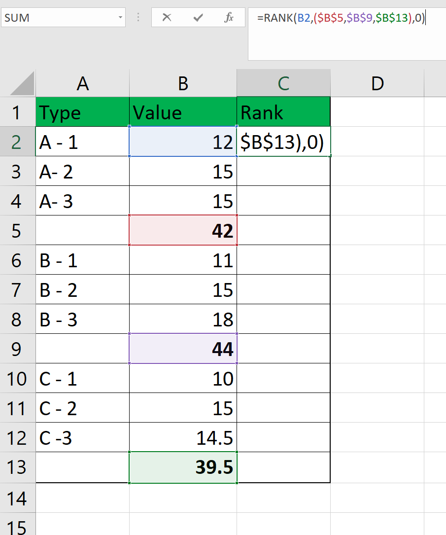
In the example below, we have a table with a list of values and their corresponding type. Each fourth cell in column B is the sum of the previous three values. Is it possible to output the rank of these summations to know which type among the three has the highest value?
![]()
The RANK function’s second argument can simply be a list of non-continuous cells. If we provide cells B5, B9, and B13 as our second argument, we can find out the rank of each cell against each other.
Now that we’ve described an example where we’ll need to use the RANK function on a non-continuous range, let’s explore a real working example in Excel.
A Real Example of Ranking Non-continuous Ranges in Excel
Let’s take a look at a real example of the RANK function being used in an Excel spreadsheet.
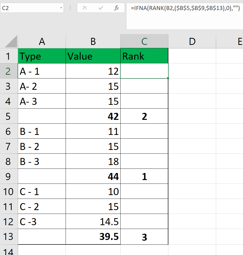
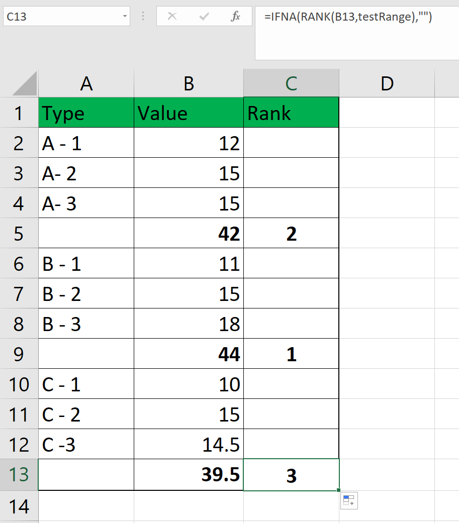
In the example below, we’ve used the RANK function to compute the rank of three cells. We’ve also used the IFNA function to ignore any #N/A errors for cells with values outside the three we’re interested in.
![]()
To get the values in Column C, we just need to use the following formula:
=IFNA(RANK(B13, testRange), “”)
The ‘testRange’ argument is a named range that refers to the cells B5, B9, and B13. In the next section, we will explain how to create your own named non-continuous range.
You can make your own copy of the spreadsheet above using the link attached below.
If you’re ready to try out the RANK function in Excel with non-continuous ranges, let’s start writing it ourselves!
How to Rank Non-Continuous Range in Excel
This section will guide you through each step needed to start using the RANK function in Excel. You’ll learn how we can use the RANK function to rank cells in a non-continuous range.
Follow these steps to start ranking non-continuous ranges:
- First, select the first cell to hold our
RANKfunction. For this example, we’ll start with cell C2.

- Next, we will need to add our arguments. The first argument must be the value you would like to rank. In this example, we’ll be ranking the cell directly to the left.
The second argument will have our list of cells to rank against. Since we want these values to be fixed, we’ve added the ‘$’ to create absolute references.
Lastly, a ‘0‘ for the third argument indicates that we want our values to be ranked in ascending order. An ascending order of ranking gives the highest value a rank of 1.
- Drag down the formula to fill in the rest of the row. Since some values are not included in the list of values to rank against, some cells will return a #N/A error. We will try to fix this in the next step.

- To remove the #N/A error, we can wrap our
RANKfunction with anIFNAfunction. In the example below, we’ve set up our formula so that if theRANKfunction returns a #N/A error, an empty string will be displayed instead.
Alternatively, we can also give our non-continuous range a name to easily reference it in our RANK function. The following steps will show how we can accomplish this.
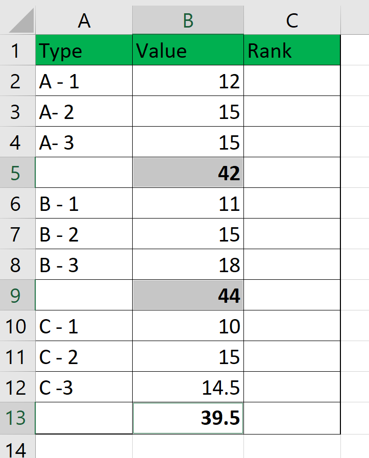
- First, select all cells to include in the non-continuous range. In this example, we’ve included cells B5, B9, and B13.
- Next, head to the Formulas tab and look for the Define Name option. Click on this button to open up the New Name dialog option.
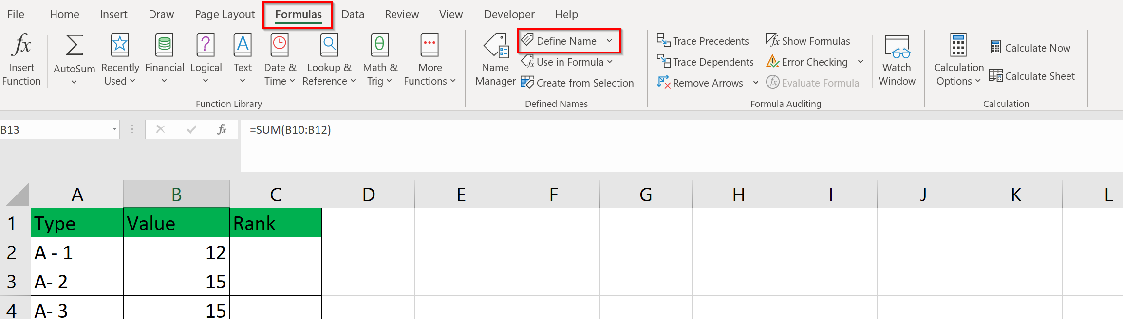
- We can now specify which cells to include in our named range in the New Name dialog. Since our cells have already been selected, it is automatically added to the Refers to input box. We can also add our own range name in the Name input box. Click on OK to set the new named range.

- We can now type in the name of our non-continuous range to our
RANKfunction.
This guide has shown you all you need to remember to start using the RANK function in Excel to rank non-continuous ranges. We’ve also shown how easy it is to convert non-continuous ranges into named ranges that are easier to reference in formulas.
The RANK function is just one of many mathematical functions in Excel. With so many other Excel functions out there, you can certainly find one that can help your use case.
Are you interested in learning more about what Excel can do? Make sure to subscribe to our newsletter to be the first to know about the latest guides and tutorials from us.