This guide will discuss how to calculate mean squared error in Excel using the AVERAGE function.
The rules for using the AVERAGE function in Excel is the following:
- The
AVERAGEfunction can only support up to 255 individual arguments which can be numbers, cell references, ranges, arrays, and constants. Furthermore, the function will ignore empty cells and cells that contain text values or logical values. - When the selected or inputted range of cells has no numeric values, the function will return a #DIV/0! error.
- However, the function will include zero values.
Since Excel contains several built-in functions and tools, it makes complicated and long calculations easier and faster. With the help of the many functions and tools, statistical calculations are quickly done and are more accurate.
For instance, calculating the mean squared error manually can take several calculations that allow more errors to occur in the process. However, calculating the mean squared error in Excel can reduce the errors and make the entire process faster.
So the mean squared error, also known as MSE is used to measure the average squared difference between the estimated or forecasted values and the actual or true values of a data distribution.
In this case, we will focus on learning how to calculate the mean squared error in Excel using its formula together with the built-in functions, such as the AVERAGE function.
Let’s take a sample scenario wherein we need to calculate the mean squared error in Excel.
Suppose you have created a sales report containing the expected or estimated number of sales and the actual number of sales for 8 consecutive sales periods or months. And you are tasked to determine the mean squared error of the data set to determine how close the estimated values are to the actual values.
To do this easier and faster, you opted to perform the calculations in Excel using the mean squared error formula and the AVERAGE function.
Before we move on to a real example of calculating the mean squared error in Excel, let’s first learn about the syntax of the AVERAGE function.
The Anatomy of the AVERAGE Function
The syntax or the way we write the AVERAGE function is as follows:
=AVERAGE(number1, [number2],...)
Let’s take apart this formula and understand what each term means:
- = the equal sign is how we activate any function in Excel.
- AVERAGE() refers to our
AVERAGEfunction. And this function is used to return the average or arithmetic mean of the selected or inputted arguments, which can be numbers or names, arrays, or cell references that have numbers. - number1 is a required argument. So this refers to 1 to 255 numeric arguments for which we want to get the average.
- number2 is an optional argument. And this acts as a supplement or additional argument that still refers to 1 to 255 numeric arguments for which we want to calculate the average.
Great! Now we can move on and dive into a real example of calculating the mean squared error in Excel.
A Real Example of Calculating Mean Squared Error in Excel
Let’s say we have a data set containing three columns. Firstly, we have the sales periods or months. Then, we have a column containing the actual values for the number of sales made for that specific month. Lastly, we have a column containing the forecasted or estimated number of sales for each month.
So our initial data set would look like this:

Since we want to calculate the mean squared error for our data set, let’s learn more about the mean squared error. So the mean squared error or also known as MSE is an estimate that measures the average squared difference between the forecasted values and the actual or true values of a data set.
However, the mean squared error calculates the average squared differences between the points and the regression line in regression analysis. In simpler terms, the mean of the squared of the residuals.
To calculate the mean squared error, we need to use the formula MSE = (1/n) * Σ(actual – forecast)^2 wherein Σ is a symbol that represents the sum, n refers to the sample size of the data set, actual means the actual data value, and forecast refers to the forecasted or estimated data value.
Additionally, the mean squared error is always positive. So the lower the value for the mean squared error, the closer the forecasted or estimated values are to the actual or true values in the data set.
If we want to ensure that our forecasted number of sales is actually closer to the actual number of sales, the mean squared error of our data set should be a really small positive value.
To apply the mean squared error formula in Excel, we will utilize the different built-in functions and features it has to make the process easier and faster. Firstly, we will calculate the squared error for each month in our data set.
To do this, we will utilize the formula =(actual value - forecast value)^2. Then, we will copy and repeat this formula for each month to get the squared error for all the rows in the data set.
Afterward, we can proceed to calculate the mean squared error using the AVERAGE function. So the average function returns the average value of the numbers within the range of cells we select or input as arguments.
And our final data set would look like this:
You can make your own copy of the spreadsheet above using the link attached below.
Amazing! Now we can move on and discuss the steps of how to calculate the mean squared error in Excel using the AVERAGE function.
How to Calculate Mean Squared Error in Excel
In this section, we will explain the step-by-step process of how to calculate the mean squared error in Excel. Additionally, each step will contain detailed instructions and pictures for you to easily follow.
To apply this method in your work, simply follow the steps below.
1. Firstly, we need to create a new column within our data set to input the squared error for each month. To do this, we will type in the formula “=(C2-D2)^2”. Lastly, we will press the Enter key to return the result.

2. Secondly, we will drag down the Fill Handle tool to apply the formula to the rest of the cells. So we can finally have the squared error for all the months in the data set.

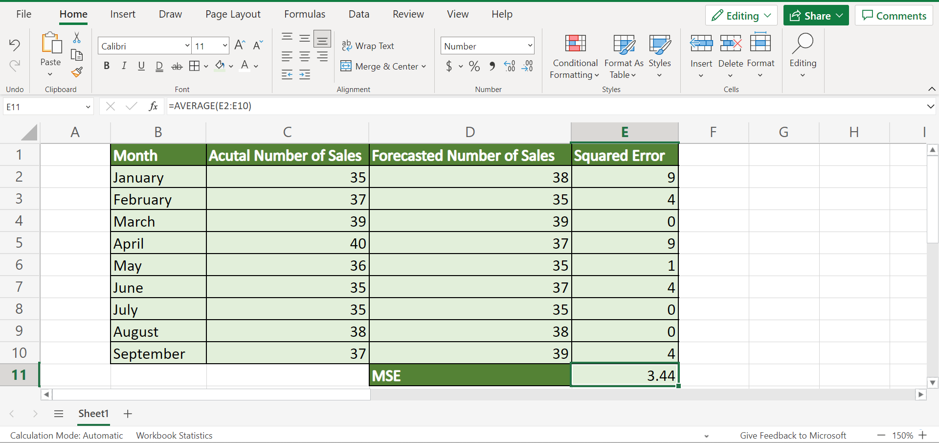
3. Thirdly, we can now calculate the mean squared error using the AVERAGE function. To do this, we will input the formula “=AVERAGE(E2:E10)”. Then, we will press the Enter key to return the result.

4. Additionally, we can choose to reduce the number of decimal points in our final result for the mean squared error. For instance, we want our mean squared error to only have two decimal points.
To do this, we can simply go to the Home tab and click the Decrease Decimal icon found in the Number section until we have two decimal points left.

5. And tada! We have successfully calculated the mean squared error in Excel.
And that’s pretty much it! We have successfully explained the step-by-step process of how to calculate the mean squared error in Excel. Now you can apply this method to your work whenever you need to calculate the mean squared error of your data set.
Are you interested in learning more about what Excel can do? You can now use the AVERAGE function and the various other Microsoft Excel formulas available to create great worksheets that work for you. Make sure to subscribe to our newsletter to be the first to know about the latest guides and tutorials from us.