


This guide will discuss how to calculate the standard error in Excel using two easy methods.
Excel is an excellent tool to use for different purposes and situations. Since it has several built-in functions and tools, we can efficiently perform complex tasks such as data analysis and analytical calculations.
For instance, we can easily calculate the standard error in Excel. So the standard error is a common calculation we encounter. And the standard error tells us how accurate our mean sample is compared to the true population mean.
Furthermore, the standard error can help us analyze how accurately our sample mean represents the true population. Additionally, we can determine the dispersion or variation in our data set or samples.
So there are two methods we can utilize to calculate the standard error in Excel. Firstly, we can use a formula using the built-in function to calculate the standard error. Secondly, we can also utilize the built-in data analysis toolpak in Excel.
Let’s take a sample scenario wherein we need to calculate the standard error in Excel.
Suppose you have conducted research using a sample of 10 people. Before you continue with your data analysis, you want to get the standard error to determine if the number of people you have in your sample is accurate enough to represent the true population.
So you simply applied a formula using the STDEV, SQRT, and COUNT functions to obtain the standard error of your sample. So the higher the standard error, the more spread out the sample is. Thus, the given mean would be an inaccurate representation of the true population mean.
Before moving on to a real example of calculating the standard error in Excel, let’s first learn the functions we will utilize.
The Anatomy of the STDEV Function
The syntax or the way we write the STDEV function is as follows:
=STDEV(number1, number2)
Let’s take apart this formula and understand what each term means:
- = the equal sign is how we start any function in Excel.
- STDEV() is our
STDEVfunction. And this function is used to estimate the standard deviation based on the given sample. Additionally, the function ignores logical values and text values in the sample. - number1 is a required argument. So this argument refers to 1 to 255 numbers corresponding to a population sample. Furthermore, we can input numbers or cell references that contain numbers.
- number2 is an optional argument. And this argument refers to the same criteria as the first argument. So this serves as a supplement argument that can be numbers or cell references containing numbers.
The Anatomy of the SQRT Function
The syntax or the way we write the SQRT function is as follows:
=SQRT(number)
Let’s take apart this formula and understand what each term means:
- = the equal sign is how we begin any function in Excel.
- SQRT() refers to our
SQRTfunction. And this function is used to return the square root of the selected number. - number is the only required argument. So this refers to the number for which we want to get the square root.
Great! Now we can dive into a real example of calculating the standard error in Excel using two easy methods.
A Real Example of Calculating Standard Error in Excel
Let’s say we have a data set containing the two samples from research. So we have two columns that each have 10 values per sample. And our initial data set would look like this:

When we conduct research or survey, we do not usually work with data from the entire population. And we simply use different sampling techniques to obtain a sample from the population and use that sample instead.
However, this means we have to check how accurately our sample mean represents the true population mean. To do this, we calculate the standard error. And the standard error can also tell us the amount of dispersion or variation our data samples have.
Furthermore, the standard error is calculated by dividing the standard deviation by the square root of the sample size. Luckily, we can use two easy methods to calculate the standard error in Excel.
Firstly, we can apply a formula using the STDEV, SQRT, and COUNT functions. So the STDEV function will calculate the standard deviation of the sample. Then, the SQRT and COUNT function will return the square root of the sample size.
Secondly, we can also utilize the data analysis toolpak in Excel. Next, we simply choose the descriptive statistic option and it will return several descriptive metrics about the selected sample, including the standard error.
So our final data set would look like this:

You can make your own copy of the spreadsheet above using the link attached below.
Amazing! Now we can proceed and discuss the steps of how to calculate the standard error in Excel using two easy methods.
How to Calculate Standard Error in Excel
In this section, we will discuss the step-by-step process of how to calculate the standard error in Excel. Furthermore, each step has detailed instructions and pictures to guide you along the way.
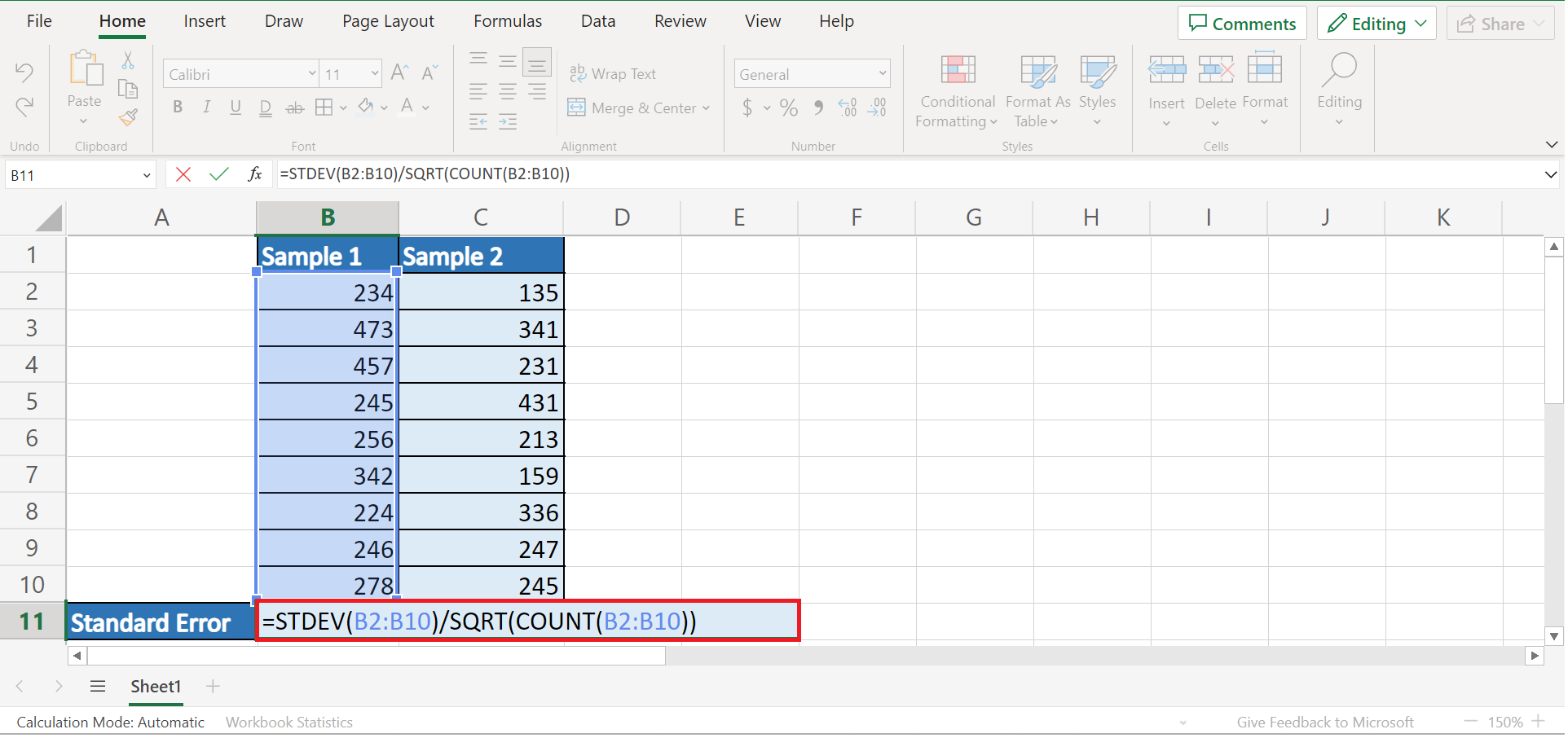
1. Firstly, we will apply a formula to calculate the standard error of our sample. To do this, we can simply input the formula “=STDEV(B2:B10)/SQRT(COUNT(B2:B10))”. Lastly, we will press the Enter key to return the result.
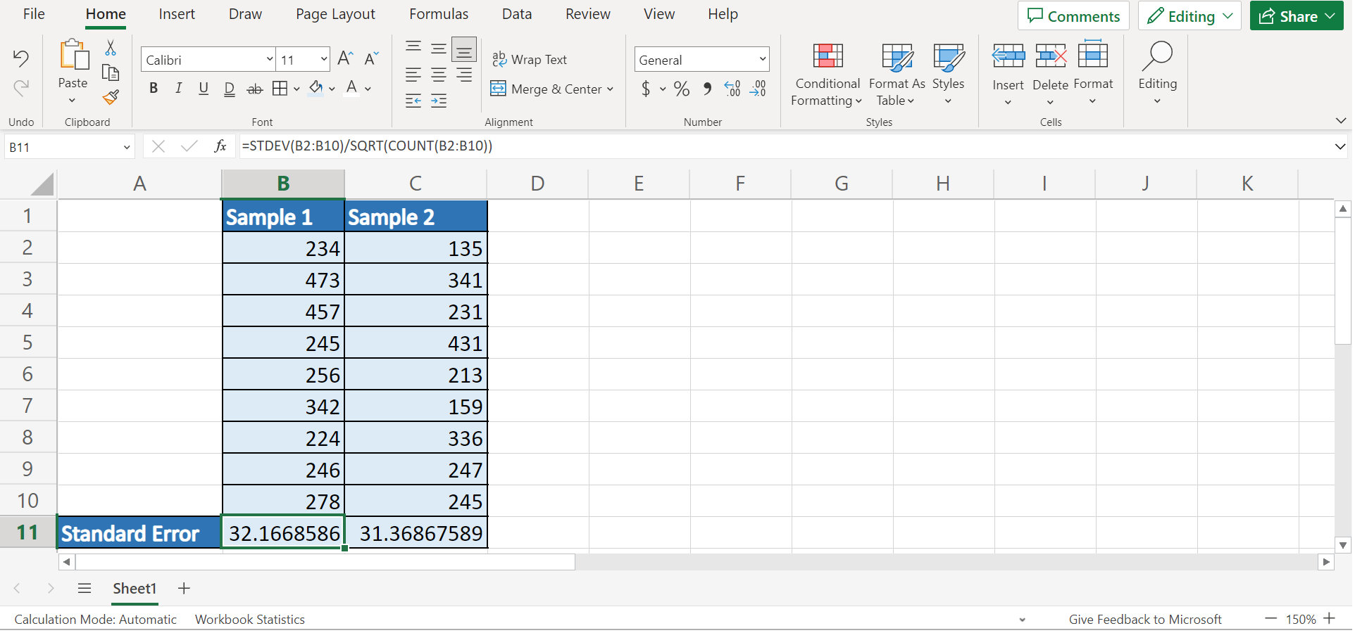
2. Secondly, we will drag the Fill Handle tool to the right to apply the same formula to our second sample.
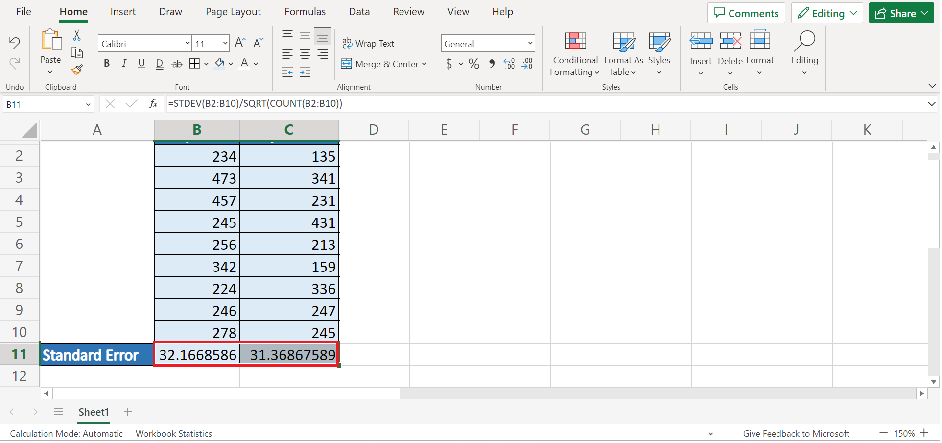
3. And tada! We have successfully calculated the standard error in Excel using a formula.
4. Alternatively, we can utilize the data analysis toolpak in Excel. If you do not have this yet, let us first install it. To do this, we will go to the File tab and select More. Next, we will choose Options.

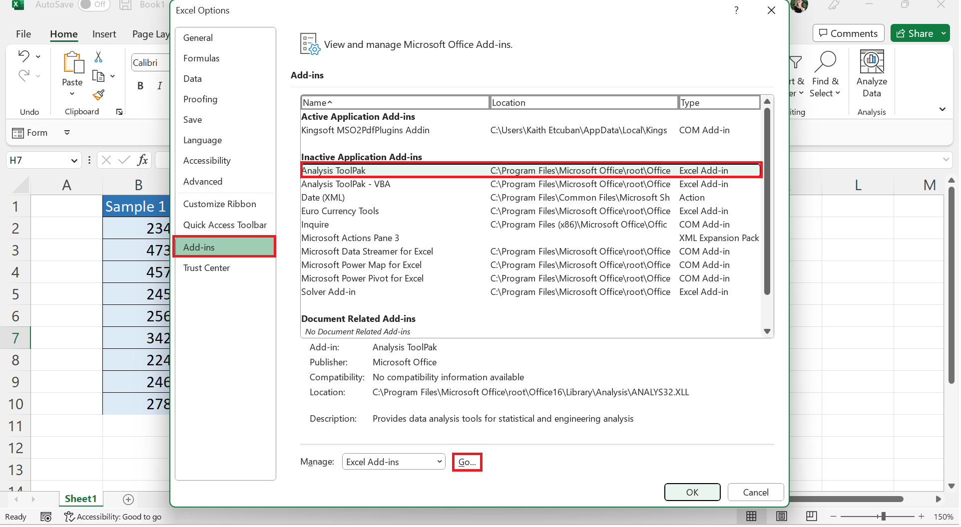
5. Then, we will click Add-ins which is found on the left side of the window. Next, we will select Analysis ToolPak from the list of Add-ins. Lastly, we will click Go.
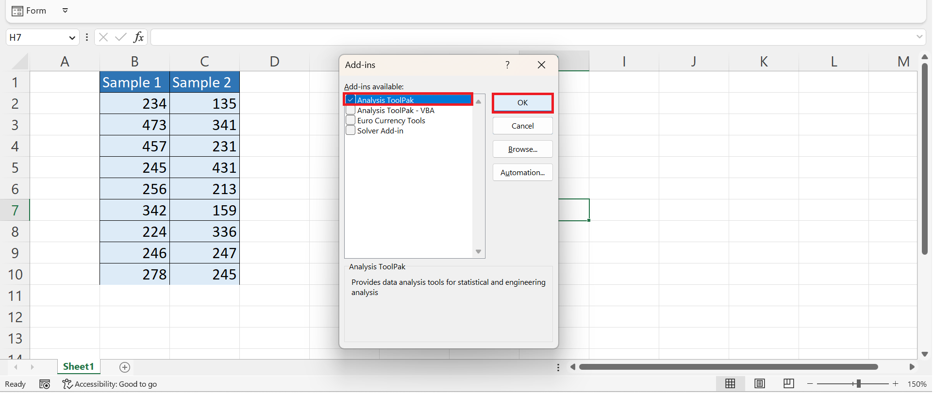
6. Finally, we will choose Analysis ToolPak and click OK.
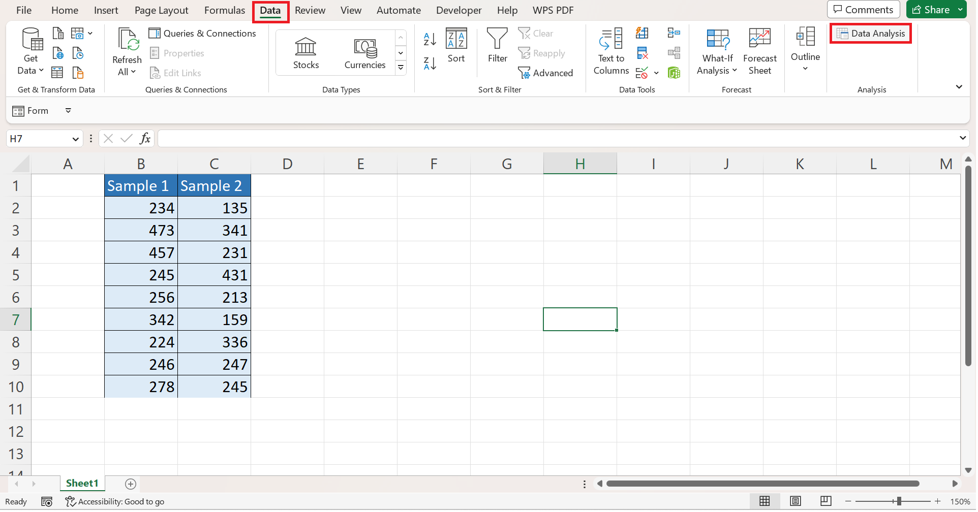
7. Afterward, we will go to the Data tab and select Data Analysis.
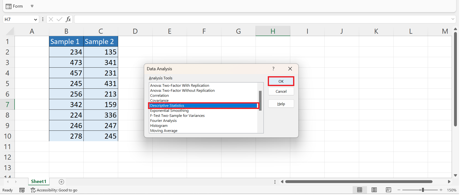
8. In the Data Analysis window, we will choose Descriptive Statistics and click OK.
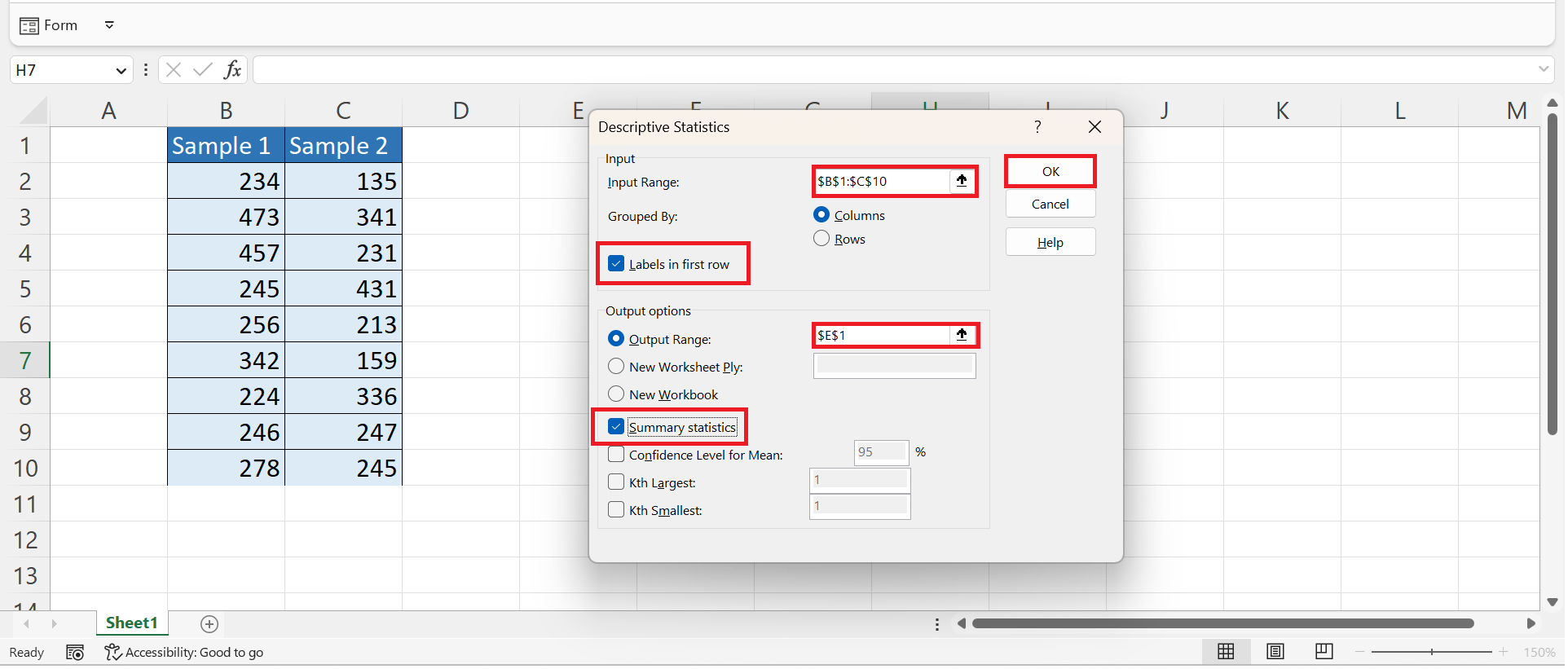
9. Next, we will input the location containing our sample in the Input Range box. Then, we will check the box for Labels in the first row. After, we will input the location where we want to display the results. Lastly, we will check the box for Summary Statistics and click OK to apply everything.
10. And tada! We have obtained the standard error in Excel.
And that’s pretty much it! We have discussed how to calculate the standard error in Excel using two easy methods. Now you can simply choose one of the methods and apply them to your work.
Are you interested in learning more about what Excel can do? You can now use the STDEV function and the various other Microsoft Excel formulas available to create great worksheets that work for you. Make sure to subscribe to our newsletter to be the first to know about the latest guides and tutorials from us.


