How to Use the CHOOSE Function in Excel

This guide will explain how to use the CHOOSE function in Excel.

When setting up a spreadsheet, you may encounter scenarios where you want a formula to return a different value or calculation depending on a specific input.

The CHOOSE function in Microsoft Excel allows you to select from a list of values given a specific index number. This can be a more efficient way to create conditional formulas without having to rely on nested IF statements.

In this guide, we will provide a step-by-step tutorial on how to use the CHOOSE function to determine the values to output in a specific cell.

The Anatomy of the CHOOSE Function

The syntax of the CHOOSE function is as follows:

=CHOOSE(index_num, value1, [value2], ...)

Let’s look at each argument to understand how to use the CHOOSE function.

• = the equal sign is how we start any function in Excel.
• CHOOSE() refers to our CHOOSE function. The function allows us to return a value of a given index number from a list of value arguments. For example, given a list of 10 values, we can specify our formula to return the fifth argument by setting the index_num value to 5.
• index_num is the argument that determines which value argument to select.
• value1, [value2], … are the value arguments to choose from.
• If index_num is equal to 1, CHOOSE returns value1. If index_num is 2, CHOOSE returns value2 and so on.
• The value arguments can be any type of value. These arguments can also be cell references as well.
• Providing an index number less than 1 or greater than the number of values provide will result in an error.

A Real Example of Using the CHOOSE Function in Excel

Let’s explore a simple example where we can use the CHOOSE function to select from a list or range of values.

Using CHOOSE With Multiple Value Arguments

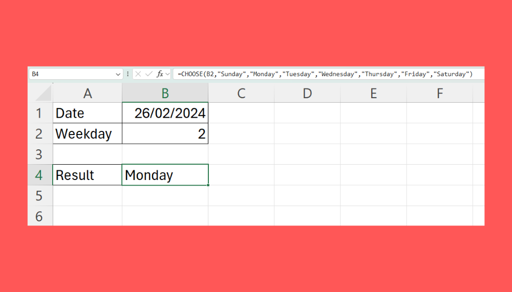
In the table above, we have a formula in cell B2 that returns the weekday of the date entered in cell B2. The WEEKDAY formula returns an integer from 1 to 7 that corresponds to a particular day of the week. For example, a value of 1 implies a Sunday, a value of 2 is equal to Monday, and so on.

To convert these integers into an actual weekday, we can use the following formula:

=CHOOSE(B2,"Sunday","Monday","Tuesday","Wednesday","Thursday","Friday","Saturday")

The first argument should be the cell containing the day of the week. The remaining arguments should correspond with the value to return if the first argument is equal to 1, 2, and so on. Since 1 is equal to Sunday, we’ll start our list with “Sunday” and proceed with the rest of the weekday names in order.

In the example above, we used the CHOOSE function to identify that the date “26/02/2024” falls on a Monday.

Using CHOOSE To Perform Different Calculations

The CHOOSE function also allows us to decide what operations to perform depending on certain conditions.

The table above shows what discounts to apply depending on the quantity of items purchased in a single order. For example, an order with an item quantity of 1000 will have a 20% discount deducted from the total amount.

To fill in column D in the table above, we can use the following CHOOSE formula:

=CHOOSE((B2>0) + (B2>=100) + (B2>=500) + (B2>1000),C2,C2*0.95,C2*0.9,C2*0.8)

The first argument consists of multiple conditions that evaluate a number from 1 to 4 depending on the value in cell B2. The remaining arguments consist of equations to evaluate depending on the result of the first argument.

For example, order 101 has a total quantity of 616 which requires a discount of 10%. The CHOOSE function returns the third choice (C2*0.9) since our first argument will evaluate to 3 (all conditions are true except for B2>1000).

Click on the link below to create your own copy of our examples.

Head to the next section to read our step-by-step tutorial on how to use the CHOOSE function in Excel.

How to Use the CHOOSE Function in Excel

1. First, select an empty cell where you want to output the result of the CHOOSE function.
   
   In this example, we’ll use the CHOOSE function in cell B4.
   
2. First, select an empty cell where you want to output the result of the CHOOSE function.
   
   In this example, we’ll use the CHOOSE function in cell B4.
   
3. First, select an empty cell where you want to output the result of the CHOOSE function.
   
   In this example, we’ll use the CHOOSE function in cell B4.
   
4. Type “=CHOOSE(“ to start the CHOOSE function in the selected cell.
   
   For the first argument, type an integer to use as the index number. Alternatively, you can add a cell reference that will contain the desired index number.
   
5. All remaining arguments after the first argument should contain the values to choose from. They must be entered as separate arguments.
   
   In this example, we’ll type the days of the week starting from “Sunday” until “Saturday”.
   
6. Hit the Enter key to evaluate the function.
   
7. If the CHOOSE function returns a #VALUE! error, the index number may be less than 1 or over the total number of provided options.
   

FAQs

1. How many arguments can the CHOOSE function take?
   Microsoft Excel allows up to 254 value arguments to input from which CHOOSE will select from. These arguments can be numerical data, cell references, formulas, text, and defined names.

To learn more about using Excel for handling multiple conditions, you can read our post on how to use an IF function with three conditions in Excel.

That’s all for this guide! Be sure to check out our library of spreadsheet resources, tips, and tricks!