How to Combine Two Query Results in Google Sheets

MeThis guide will explain how to combine two query results in Google Sheets.

The QUERY function is a convenient way to filter your data based on certain criteria. If you find the need to combine two or more QUERY results into a single formula, Google Sheets provides a way to do so.

Let’s take a look at a quick example! 

Suppose you have a list of credit card payments made by users around the world. Using the QUERY function, you set up two queries to fill two separate tables. The first query returns a list of transactions you need to refund. Meanwhile, the second query returns a list of payments that you’ve charged the incorrect amount.

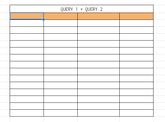
You want to replace these two tables with a single table that combines the results of both of these queries. How can we do this with a single formula?

If you need to combine two ranges vertically in Google Sheets, you can use the semicolon symbol and curly braces. Google Sheets allows users to combine multiple cells or arrays together using commas, semicolons, and curly braces.

Now that we know when we might need to combine query results, let’s look at a sample spreadsheet that uses array syntax to perform this.

A Real Example of Combining Two Query Results in Google Sheets

Let’s explore a real example of a Google Sheets spreadsheet that combines query results using a single formula.

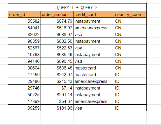
In this example, we have a spreadsheet with various credit card transactions. Each transaction is given a unique order ID. Each entry in our table contains the transaction’s country code, the amount in dollars, and the time the transaction was made.

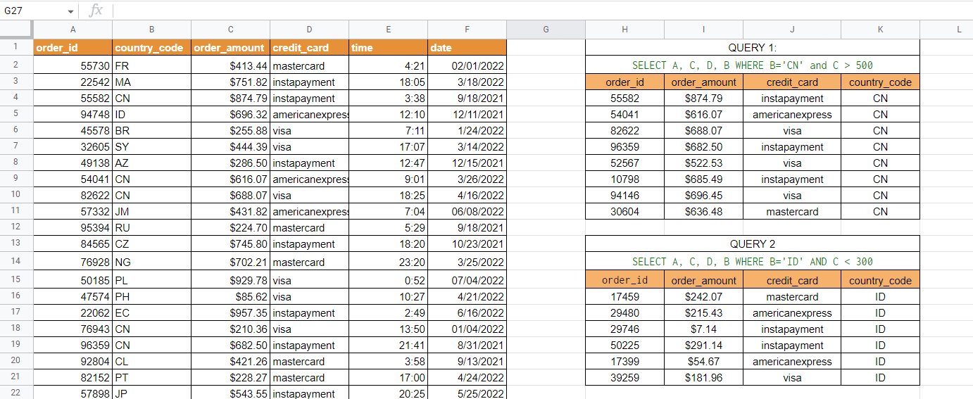
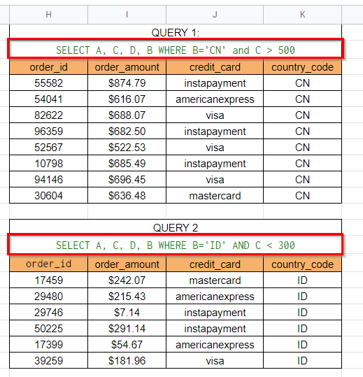
Our spreadsheet already uses two queries. The first query flags transactions from China with an order amount greater than $500. The second query flags transactions from Indonesia with an order amount of less than $300. We want to combine these two query results into a single table.

To get the values in the table above, we just need to use the following formula:

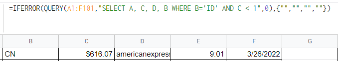
={IFERROR(QUERY(A1:F101,"SELECT A, C, D, B WHERE B='CN' and C > 500",1),{"","","",""});

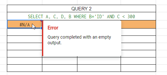
IFERROR(QUERY(A1:F101,"SELECT A, C, D, B WHERE B='ID' AND C < 1",0),{"","","",""})}

Using the array syntax, we can specify that we want to combine these two results vertically using a semicolon. Since we’re treating these results as array elements, we’ll need to start and close our formula with curly braces. 

Note that combining two arrays vertically requires both of them to have the same number of columns.

Since the QUERY function returns an error if no results are found, we’ll have to catch that error using the IFERROR function. If either function returns an error, the error will be replaced with an array of empty strings. The array should have the same length as the number of columns you were supposed to output.

You can make your own copy of the spreadsheet above using the link attached below. 

If you’re ready to try combining two query results in Google Sheets, let’s begin writing it ourselves!

How to Combine Two Query Results in Google Sheets

This section will guide you through each step needed to combine two query results in Google Sheets. You’ll learn how we can use curly braces and a semicolon to merge two output arrays vertically.

Follow these steps to learn how to combine two query results:

1. First, determine the query strings you need for the two formulas you want to merge. For instance, we’ll retrieve our formulas in this example from two existing tables in our spreadsheet.
   
2. Select the cell that will contain our combined QUERY functions.
   
3. Next, create a new formula that combines both QUERY formulas separated by semicolons. After that, wrap the entire formula with curly braces.
   
4. Hit the Enter key in order to return the combined result.
   
   

You may find a #N/A error if any of the two QUERY formulas return no results. To fix this issue, we can modify our formula slightly.

1. We’ll use the QUERY function as the first argument to the IFERROR function. In case our query returns an error, we can return instead an array of empty strings. The array should have the same number of elements as there are columns in the original query.
   
   
   
2. We can apply this modification to both QUERY functions in our final formula.
   
   

This step-by-step guide should be all you need to know to start combining two query results in Google Sheets. Our guide shows how you can use array syntax to vertically merge the output of two QUERY functions.

The QUERY function is undeniably a powerful function you can use to explore your data in Google Sheets. Because the function comes with its own built-in query language, many users rely on it to filter their data using a single formula.

As seen in our modified formula, the QUERY function can also be used together with conditional functions like IFERROR. With so many other Google Sheets functions available, you can surely find one that suits your use case. 

Are you interested in learning more about what Google Sheets can do? Subscribe to our newsletter to find out about the latest Google Sheets guides and tutorials from us. 

Get emails from us about Google Sheets.

Our goal this year is to create lots of rich, bite-sized tutorials for Google Sheets users like you. If you liked this one, you'd love what we are working on! Readers receive ✨ early access ✨ to new content.

Subscribe