How to Copy a Formula Down an Entire Column in Google Sheets

You can easily copy a formula down an entire column in Google Sheets to automate your work and save a lot of time.

When using a spreadsheet, you often need to apply a formula to an entire column or row.

If you have a hundred or a thousand cells in a column, you can’t manually apply a function to each cell.

Let’s take an example.

Say you want to do the same mathematical calculation to a long list of numbers. For example, compute the square of many numbers.

Writing the formula in every cell one by one would be too exhausting and takes a lot of time.

Fortunately, there are diverse ways to copy a formula down to an entire column in Google Sheets without manually entering them:

• Dragging down the fill handle tool
• Double-clicking the fill handle tool
• Using the ARRAYFORMULA function

In this guide, I’ll show you how you can use each of these methods.

Let’s dive right in. 🤜

1. Using the Fill Handle to Copy a Formula Down an Entire Column

The easiest approach to copy a formula down is to use the so-called fill handle.

The fill handle is a feature in Google Sheets that can apply a formula to an entire column. You can manually drag the fill handle if you have a smaller dataset.

The picture below shows a list of numbers in column A, and we display the square of these numbers in column B.

Let’s see step-by-step how can we use the fill handle to copy the formula down the entire column.

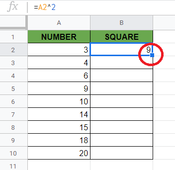
1. To start, we select the upmost cell of the column and write the formula in it. The function we write in cell B2 is a formula to calculate the square of the cell A2:

=A2^2

2. Then, we point our mouse to the bottom-right corner of the formula cell. There is a little blue square there that is the fill handle. While moving the cursor to the fill handle, it should change to a black plus icon.

3. We click and drag the fill handle downwards until reaching the lowest cell where we want to apply the formula. We do this by holding the left click until we reach the end of the column.

After using the fill handle, the other cells in the column have the same function. The cell references are relative. This means that the fill handle automatically adjusts the references according to the cell position.

Look at the picture below to understand this better.

For example, in the fourth row, we would like to compute the square root of A4, but our original function has a reference to this cell A2.

Don’t worry, since Google Sheets manages this for us automatically.  While the function in cell B2 has a reference to A2, B3 has a reference to A3, B4 has a reference to A4, and so on.

It always shows the correct result of each row, and we didn’t have to type them manually.

It’s so easy, right?

Try it out by yourself. You may make a copy of the spreadsheet using the link I have attached below:

2. Double Clicking on the Fill Handle to Copy a Formula Down an Entire Column

You can achieve the same result as above by double-clicking on the fill handle.

It will automatically find the end of the column and fill the column with the same formula until the last filled cell.

This is an even faster way to copy a formula down an entire column. It doesn’t require you to drag down the entire column with your mouse.

But be aware that this method cannot be used in every sheet. While it’s very automatic and saves a lot of time, it also has limitations.

In case you have an empty cell in your column, the formula will stop right before that. It will detect the empty cell as the end of your column, so the formula will not be applied to the rest of the column.

Look at the example below where we have the same formula in the first row as before. The table has an empty cell in the middle of the column.

When we double-clicked on the fill handle, it only copied the formula down until cell B5 because Google Sheets detects it as the last filled row.

If you have empty cells in your column and don’t want to remove or fill them, it’s better to use the drag-down method shown above.

3. Using the ARRAYFORMULA Function to Copy a Formula Down an Entire Column

Another quick and effective method to copy a formula down an entire column in Google Sheets is by using the ARRAYFORMULA function.

The fill handle is suitable for smaller columns. However, if you have a massive table, it might be better to apply the formula with the use of the ARRAYFORMULA function.

The ARRAYFORMULA function is useful to fill the formula in the entire column while we only need to put a formula in the first cell. It is a single formula that can fill our entire column without having to copy or drag down multiple formulas.

We have explained in details how to use ARRAYFORMULA function in Google Sheets in our previous article. Check it out to learn more about its syntax and use cases!

But now let’s see step-by-step how to use it in our previous example to apply the square formula to an entire column.

1. As before, we start by selecting the upmost cell of the column. This is where we type our ARRAYFORMULA function, and it’s again the cell B2 in our example.

2. We added our function in this cell. To start, we put an ‘=’ equal sign, followed by the name of the function ‘ARRAYFORMULA‘ and an opening bracket.

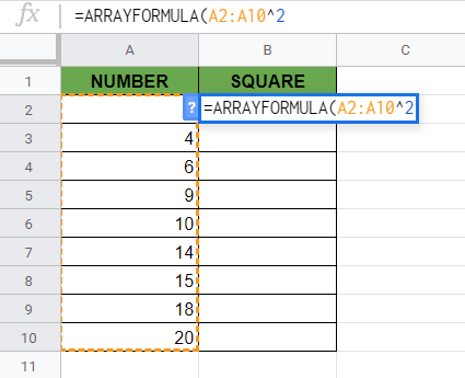
3. After that, we write the calculation we need into it. When using the ARRAYFORMULA function, we wrap our original function. But we also have to change the single-cell references in our formula into references that refer to a range of cells. In this case, instead of specifying a single cell as a parameter (A2), we’ll specify the entire range of cells whose square we want to calculate (A2:A10).

4. Finally, we compute the squares. In Google Sheets, we do it with adding ‘^2’ after the cell references. The whole function we write in cell B2 is as follows:

=ARRAYFORMULA(A2:A10^2)

5. As a result, the ARRAYFORMULA function applies the same calculation to the entire column. It does so until the row we specified in the range reference which is the cell A10 here. But we could apply the same formula to even thousands of cells.

⚠️ A Few Notes to Use the ARRAYFORMULA Method Even Better:

1. Here we typed the name of the ARRAYFORMULA function. Instead, you can also convert a regular function to an ARRAYFORMULA with key shortcuts. Press Ctrl+Shift+Enter on Windows or Cmd+Shift+Enter on Mac to automatically wrap your formula with the ARRAYFORMULA function.
2. We can apply a formula to the entire column of the sheet with only a single cell with a formula in it. It’s easier to maintain as you only need to change one cell to edit the calculation.
3. While this is powerful, it has a weak point too. If you delete this single cell, the whole referred column will be deleted.
4. You cannot delete just a single cell from the column with this method. If you try to delete the content of a cell in the middle that is part of the array, nothing will happen.

That’s pretty much it. Now you know how to copy a formula down an entire column together with the various other Google Sheets formulas to create even more powerful formulas that can make your life much easier. 🙂

Get emails from us about Google Sheets.

Our goal this year is to create lots of rich, bite-sized tutorials for Google Sheets users like you. If you liked this one, you'll love what we are working on! Readers receive ✨ early access ✨ to new content. There will be no spam and you can unsubscribe at any time.

Subscribe