How to Count If Not Blank in Google Sheets

To count if not blank in Google Sheets is useful if you want to count the cells that just have data in it (not blank).

The technique is commonly used when you have to count a specific cell range, especially if you have a large number of cells and you want an accurate count of the cells which are not blank.

For instance, you are running a small supermarket with 200 different items. You listed all the names of the items in Google Sheets. Using the techniques shared below, you can precisely obtain the right amount of stock ignoring cells that are blank and useless.

Ready to get started? Let’s dive right in! 😊

How To Count If Not Blank in Google Sheets: 3 Ways

1. Using COUNTA Function.

For the first approach when counting if not blank cells, we will be using the COUNTA (Count All) Function.

The syntax or in other words the way we write the function is as follows:

=COUNTA(value1, [value2, ...])

Let’s break this COUNTA function down:

• = denotes the start of every formula written in Google Sheets.
• COUNTA() is our function of which we need to provide its corresponding value.
• value1 we have to select the cell range that we want to count. This value is required to be given and the function will not work without it.
• value2 , and subsequent attributes ‘...‘ are additional cells to be included in the count. The maximum number of entries allowed is 30.

It’s a good idea to have some understanding of how to use the COUNTA function in Google Sheets before delving into using COUNTA to count if not blank cells.

Now the big question in your mind at this point is, “what’s the use of learning this function?”

Well, when you are really sure that all your cells are blank, you can use the COUNTA function to count the cells which are not blank.

Let’s take an example.

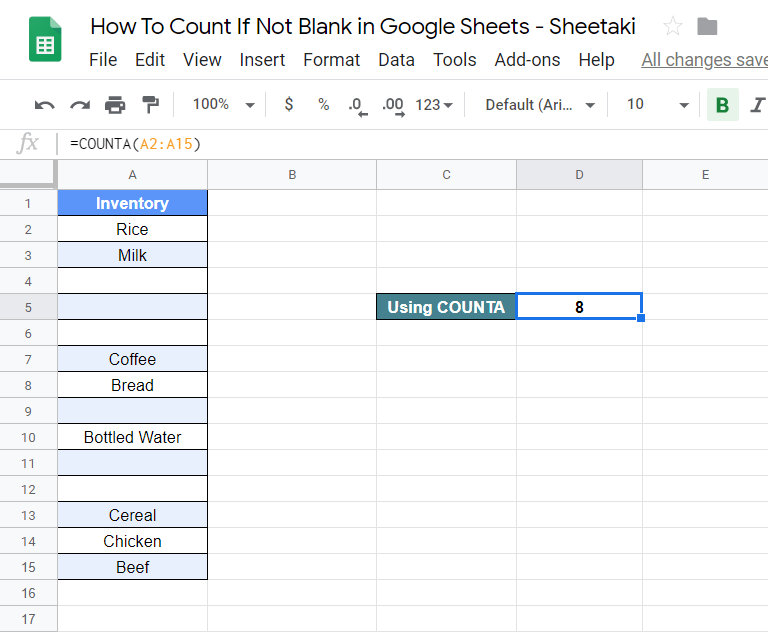
In the image below, cells A4:A6, A9, A11:A12, and A16 are empty. Using our finished COUNTA function which is =COUNTA(A2:A15) it will result in an answer of 8 which is correct as there are only eight cells which are not blank as shown below:

When you’re unsure of cells being blank, such as if you may have mistakenly entered an apostrophe or space in any of the cells, then COUNTA will count that too.

This is where COUNTA is not ideal and the other solutions shared in this guide help circumvent.

In such a case, it’s best we rely on the COUNTIF function in Google Sheets which we will show you how below. 🙂

2. Using COUNTIF Function.

As aforementioned, using the COUNTIF function is perhaps the best solution to counting cells that are not blank in Google Sheets.

It’s not uncommon to find ourselves committing little errors when typing or inputting data in our spreadsheets. There might be cases where we hit the space bar on a cell, then pressed enter without knowing. Or maybe thought to add a text, added an apostrophe, but you left it that way. In such instances, using the COUNTIF function will definitely accurately provide us the right count for cells that are not blank.

I’ll give you an example below.

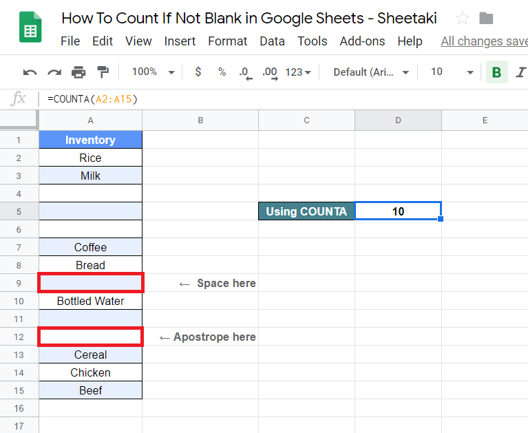
When you typed in an apostrophe and left it that way, it won’t actually register on Google Sheets, but it’s there. In other words, it’s “as if” empty.

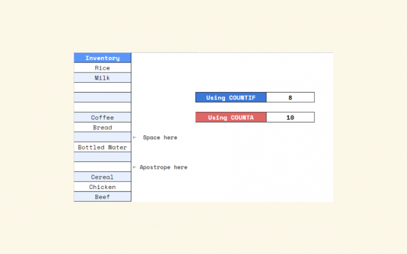
As you can see in the example above, I typed in a space on cell A4 and an apostrophe on cell A11. Instead of having an outcome of 8, it gave me a result of 10. Meaning, the COUNTA function included the space and the apostrophe in the count.

This is a clear picture of a situation where the COUNTIF function fares well.

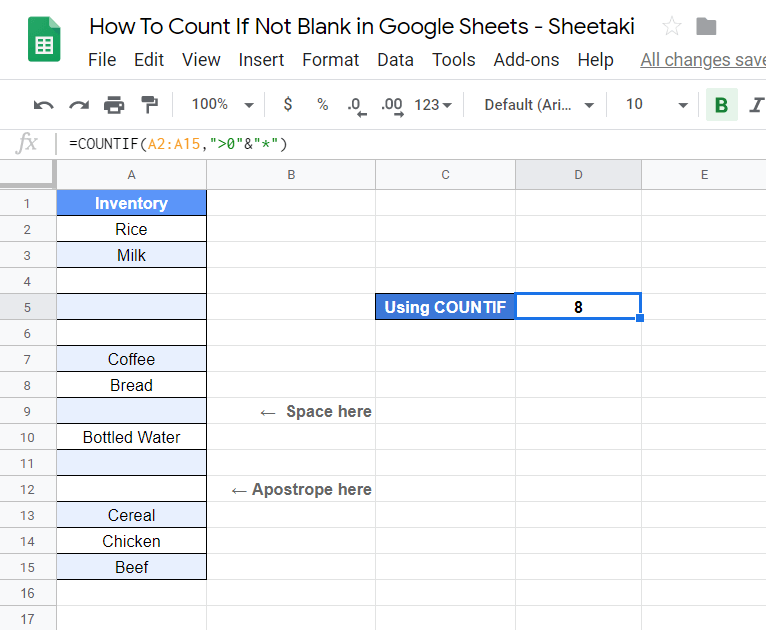
We can use the COUNTIF formula as shown below:

=COUNTIF(A2:A15,">0"&"*")

Let’s break this COUNTIF function down to understand how it works:

• = denotes the start of every formula written in Google Sheets.
• COUNTIF() is our function. We need to add other attributes for it to work smoothly.
• range is the group of cells that the function is to search. For our example, we will be using A2:A15 as the range which contains the cells we want to count.
• criterion is the condition where each cell in the range is to be tested whether it is to be true or false. For this we provide the following:
  • ">0" is a comparison operator which means “greater than 0”. In this case, we want to say that the criterion should be that anything that is lesser than 0 should be avoided. You probably learned this from the previous COUNTIF post.
  • & is called ampersand and it merges the comparison operator and the asterisk.
  • "*" is called a wildcard character and represents or take the place of any number of characters. This is useful as we need to avoid counting unnecessary characters which are not blank such as, for example, apostrophes, full stops, commas, or even spaces.

After applying the COUNTIF function, we manage to obtain the correct count of cells which is 8 ignoring the spaces and unwanted characters which appear as blank cells.

⚠️ Now a few notes about the difference between COUNT and COUNTA

The COUNT function is commonly used when counting a range of cells that includes numbers and dates. It doesn’t count blank cells.

On the other hand, COUNTA function counts numbers, texts, dates, characters and even spaces.

⚠️ A few more notes when using these formulas

• The COUNTA function is used when the data is perfect, meaning, with no unnecessary characters like apostrophe and space.
• When using the COUNTIF function, make sure to supply the necessary attributes such as the comparison operator, the ampersand, and the asterisk. Provided so will allow your function to filter out cells that are not blank but appear as blank in your spreadsheet.

3. Using SUMPRODUCT Function.

The third solution to use is to utilize the SUMPRODUCT function and it works great at counting non-empty cells.

To make use of it we will need to provide it two other extra functions too which are the LENand TRIM functions. Doing so will allow the SUMPRODUCT function to ignore cells that may have null string or spaces as well as unwanted characters such as apostrophe being counted.

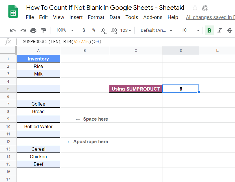
We can use the SUMPRODUCT formula as shown below:

=SUMPRODUCT(LEN(TRIM(A2:A15))>0)

Again let’s break this down:

• = required to start the function.
• SUMPRODUCT() works by calculating the sum of products of the entries. In this case, since we only provide one entry which is A2:A15 and not separated by a comma.
• LEN() is responsible to make sure each cell is inspected to see if there is at least one character or number in it. In other words, the length of the characters will have to be >0 (greater than 0). If not, it will be avoided.
• TRIM() makes sure that any spaces are ignored.
• >0 as mentioned, the length of characters will have to be greater than 0 in order to be considered. If not it is not counted and is considered blank.

When combined and implemented, the function will also provide a count of 8 just like COUNTIF did.

However, even though the SUMPRODUCT function avoids hidden characters and spaces entered in the data from being counted, the one caveat is that it does count numbers and characters such as brackets, apostrophes, commas, etc. which are included as part of the data as well.

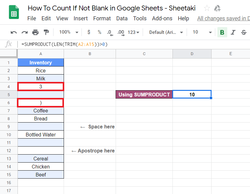
In this case, you will need to resort back to using the COUNTIF function if you really want to avoid such characters from being counted.

How to Count If Not Blank in Google Sheets Using COUNTIF

You can follow along in this section to write your own function to count non-empty cells in Google Sheets. Since COUNTIF is the more robust out of the three solutions discussed above, we will be using it instead.

We begin as follows:

1. First, click on any cell and make it active. For this guide, I will be choosing D5.

2. Next, we enter =COUNTIF followed by an opening parenthesis ‘(‘ to begin our function.

3. Now for the first attribute which is our range, we will select the enter A2:A15, as this is the cell range that we want to count.

4. Next, after entering the comma ‘,‘ we provide the criterion to evaluate the range we had already provided. For this criterion, we enclose in a quote-unquote symbol (“”), we will write greater than zero, or “>0“. Remember this is to count cells that are greater than 0 as we want to say that the cells which are lesser than 0 should be avoided.

5. After this, we will add an ampersand ‘&‘ to connect our first criterion with our second criterion. You do not have to enter a comma ‘,‘ here.

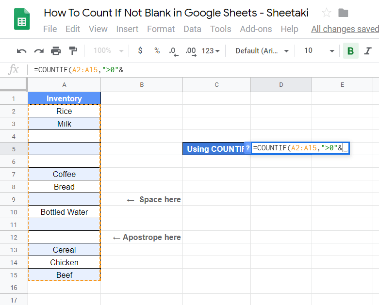
6. Now we provide the second criterion for which we type in the asterisk ‘*‘. This is to ignore characters that we may accidentally input in the cell range which appear as blank cells.

7. Finally, enter the closing parenthesis ‘)‘ and hit the Enter key to obtain the final result.

That’s it. Well done! 👏🏆

You may make a copy of the spreadsheet using the link I have attached below:

Have a feel on how to work with this formula. Try it out for yourself.

That’s pretty much it. You now know how to count if not blank in Google Sheets. Try experimenting it together with the other numerous Google Sheets formulas to create even more powerful formulas that can make your life much easier. 🙂

Get emails from us about Google Sheets.

Our goal this year is to create lots of rich, bite-sized tutorials for Google Sheets users like you. If you liked this one, you'll love what we are working on! Readers receive ✨ early access ✨ to new content.

Subscribe