How to Get Column Letter in Google Sheets

The guide is useful if you want to convert a column number to a column letter.

For example, column #5 in Google Sheets is also column E.

Even though the column letters are shown in the top row, there are no functions formulated solely to convert a column number to a column letter. 

Unlike the COLUMN function, which can get a column number of a specific cell.  

In this guide, we will go through two combinations of functions in Google Sheets that will enable you to convert a column number to a column letter. 

Mainly:

1. SUBSTITUTE + ADDRESS
2. REGEXEXTRACT + ADDRESS

 

 

Short Run Down on ADDRESS Function

The function returns a cell reference or address as a text or string as per the specified row and column numbers. 

The way we write the ADDRESS function is: 

=ADDRESS(row, column, [absolute_relative_mode]) 

Let us help you understand the context of the function:

• The row is the row number of the cell reference.
• The column is the column number of the cell reference. For example, “A” is column number “1”.
• The [absolute_relative_mode] is the indicator of whether the cell reference is row or column absolute. This attribute is optional. 

Here are the references for absolute relative mode:

For more in-depth explanations and other examples to apply the ADDRESS function, do check out our article to learn more!

 

 

Get Column Letter Using SUBSTITUTE Function

The SUBSTITUTE function replaces existing text with new text.

The way we write the SUBSTITUTE function is: 

=SUBSTITUTE(cell_to_search, search_for, replace_with) 

Let us help you understand the context of the function:

• The cell_to_search is the cell you want to make the changes to. This tells the function which cell you want it to search for to make the needed changes.
• The search_for is the text you want to replace. This tells the function of which text in the cell you want to change.
• The replace_with is the text you want to replace the search_for text with.

To understand the function better, don’t forget to check our article on SUBSTITUTE function!

Let’s combine the SUBSTITUTE and ADDRESS functions.

In this case, the ADDRESS function would be the cell_to_search attribute.

 

Example 1

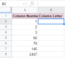
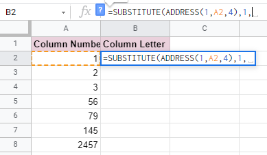
1. Simply click on the cell that you want to write down your function at. In this example, it will be B2.

 

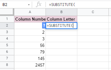
2. Begin your function with an equal sign =, then followed by the name of the function, SUBSTITUTE, then an open parenthesis (.

 

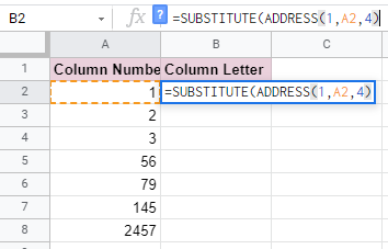
3. We will then add the ADDRESS function as the first attribute which is cell_to_search,  then add another open parenthesis (.

 

4. Then add ‘1‘ as the row and select A2 as the column. Remember to insert a comma , in between these two attributes to separate them.

 

5. Add another comma , to separate the column from the absolute_relative_mode. We then insert '4' as our reference, making its row and column relative. Close the ADDRESS function with a closing parenthesis ).

 

6. We will then input ‘1‘ as the search_for attribute. Remember to add commas , to separate the attributes from each other!

 

7. Lastly, we will insert a quote-unquote symbol "" into the formula. By not inserting any characters in between the quote-unquote symbol "", we will be replacing the ‘1″ with nothing.

 

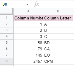
8. After the following steps, your input should look like this:

 

For those who are lost, no worries!

Let us explain how the formula is able to return with these values. 

By just looking at the ADDRESS function, the return values would look like this:

This is also similar to inputting the number as ‘3‘ instead of selecting A4 as the input for column. 

Moving on, by adding the SUBSTITUTE function, we replaced the ‘1‘ in C1. Making the end return value only showing ‘C‘.

Another thing to note, we need to input 4 as the input for absolute_relative_mode. If we were to put either 1, 2, or 3, the return value would not be only a column letter. 

Here is an example to show you what happens if we input 1 as the absolute_relative_mode.

The “1” would still be substituted with nothing. However, since 1 represents the “row” and “column” to return as absolute, the $ would appear. 

 

 

Get Column Letter Using REGEXEXTRACT Function

The REGEXEXTRACT function extracts a certain text string within a given data.

The way we write the REGEXEXTRACT function is: 

=REGEXEXTRACT(text, regular_expression)

Let us help you understand the context of the function:

• The text is the cell where you want to match a regular_expression to. In our example above, it will be A2:A8.
• The regular_expression is the word we want to match to the text.

The REGEXEXTRACT function is very useful, do check it out if you are interested!

Let’s combine the REGEXEXTRACT and ADDRESS functions.

In this case, the ADDRESS function would be the text attribute.

 

Example 1

1. Simply click on the cell that you want to write down your function at. In this example, it will be B2.   

 

2. Begin your function with an equal sign =, then followed by the name of the function, REGEXEXTRACT, then an open parenthesis (.

 

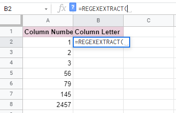
3. We will then add the ADDRESS function as the first attribute, which is text.  Then add another open parenthesis (.

 

4. Then add ‘1‘ as the row and select A2 as the column. Remember to insert a comma , in between these two attributes to separate them.

 

5. Lastly, enclosed by a quote-unquote symbol "", type in the regular expressions we want to look for. As we only want to extract the letters, we inserted only characters ‘A–Z‘ and +.

Take note that the REGEXEXTRACT function is case-sensitive. Hence, if we insert ‘a-z’ as the regular expression, it would show #N/A. This means the regular_expression we inserted could not be found in the “text”.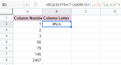

We have also added a + to signify that at least one regular_expression is required in the text or additional are optional. 

If we do not include a +, it would only extract the first letter in the text. As a result, this would make the return value look like this:

 

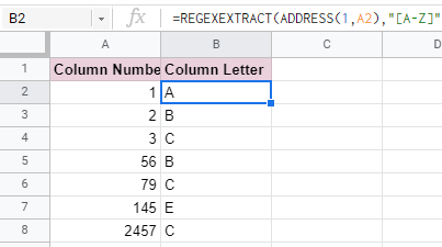
6. After the following steps, your input should look like this:

 

You may make a copy of the spreadsheet using the link attached below and try it for yourself:

Well done! Now you can easily convert column numbers into column rows! 

Be sure to check out our tutorials on other functions that use regular expressions such as REGEXEXTRACT, REGEXMATCH, and REGEXREPLACE. These tutorials will provide you much more thorough and extensive description of how a regular expression works!