How to Color Alternate Rows in Google Sheets

To color alternate rows in Google Sheets is useful if you have a large set of data, with multiple rows and columns, and want to increase its readability.

In this article, you’ll learn how to color alternate rows in Google Sheets. There is more than one way to do this, and we’ll show you all of them. After reading this article, you’ll no longer spend time on manually coloring alternate rows in your spreadsheets!

Let’s start with an example!

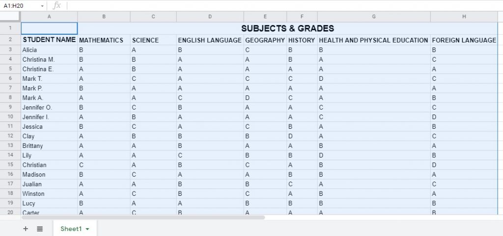
Say you’re a teacher and have a sheet with your students’ names and their grades from all of the subjects. Scrolling through the sheet to see data and keeping track of what row you’re actually looking at can be exhausting since all of the cells contain similar data (A, B, C, or D). Coloring alternate rows will help you differentiate rows, increasing the readability of the sheet and data in it. 

When rows are colored like this, they are also called ‘zebra strips’.

We’ve mentioned there is more than one way to color alternate rows in Google Sheets, so you must be wondering what those ways are?

Earlier, if you wanted to color alternate rows in a spreadsheet, you had to use conditional formatting and a custom formula. Today, you can do this more easily, with a simple built-in feature. 

Since conditional formatting can still come in handy (when you need to color every third or fourth row, or if you want to color columns), we’ll show you both ways.

Let’s start with our first method since we have a lot to cover in this article!

How to Color Alternate Rows in Google Sheets (The Simple Way)

The simple way to color alternate rows in Google Sheets involves using its built-in feature you can access from the main menu. Let’s get back to our sheet and take a quick look at how to do it!

1. First, open the sheet and select the data range in which you’d want to color alternate rows. If your sheet has a header or footer, you should include it in your selection, as well. For this guide, I’ll choose the range A1:H20.

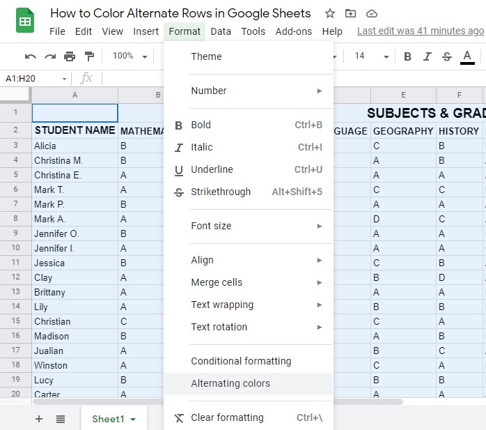
2. Then, from the top menu Format > Alternating colors. This will open the ‘Alternating colors’ toolbar on the right. Now, let’s take a look at that toolbar.

3. The top part of the toolbar, ‘Apply to range’, will show you the range you’ve selected. So, if you need to edit your selection, you can do it here. Below that, you’ll see the ‘Styles’ section. There you can select if your sheet has a header or footer. If you try it, your sheet will update automatically, so you can see how it’ll look.

4. You can choose one of the available default styles, or you can make a custom style by selecting two colors for the alternate rows, as well as the color for the header/footer if there are any.

5. Finally, click on the ‘Done’ button below or the ‘X’ in the top right corner of the toolbar, to close it and color alternate rows in your spreadsheet.

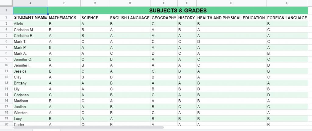
That’s it! Now you have a sheet that’s easy to scan through! 

But what if you need to color every third or fourth row or would want to color alternate columns, instead? Then you should use conditional formatting and a custom formula. Let’s show you how to do it!

How to Color Alternate Rows in Google Sheets (Conditional Formatting)

Conditional formatting should be your go-to feature when you want to change the aspect (background color or the text style) of cells, rows, or columns, based on their values and rules you set.

The rules you set are if-then statements. Each of these statements consists of a condition (if this…) and a corresponding action (then that…). This means that a certain condition needs to be evaluated, and if the condition is met, then a corresponding action will be applied to the selected range.

Let’s take a look at how to color alternate rows using conditional formatting!

1. First, you should access conditional formatting. To do this, select Format > Conditional Formatting from the main menu and the ‘Conditional format rules’ toolbar will open.

2. Select the range where you’d want to apply conditional formatting. For this guide, I’ll select A1:Z100.

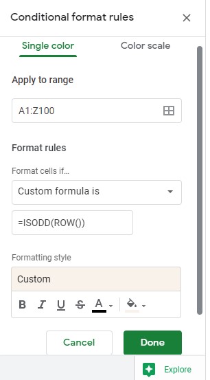
3. Now, we should set our rule. Select ‘Custom formula is’ from the drop-down list below the ‘Format cells if…’ and add the =ISEVEN(ROW()) formula to the input box

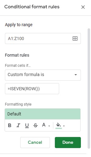
4. Select the color and you’ll see that every other row will be colored. Close the toolbar by clicking on the ‘X’ or ‘Done’ button.

Now, let’s take a quick look at the syntax of the formula and what does each of its parts means to better understand how it works!

The formula you use to apply conditional formatting is evaluated for every cell in the selected range. In our example, both =ISEVEN and the =ROW functions are run. =ROW returns the row number of the cell, while =ISEVEN returns TRUE for the even row numbers and FALSE for the odd row numbers. The formula will trigger on TRUE so that, so all even rows will be colored.

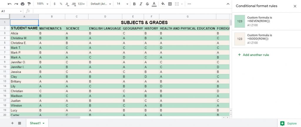
If you’d want to color the odd rows, too, you should create another rule, with the =ISODD function instead. Follow the same steps as before (or just click the ‘Add another rule’ link if the ‘Conditional formatting’ toolbar is still open) but use the =ISODD(ROW()) function and choose another color for the selection.

That’s it! Now you have set conditional formatting for both even and odd rows, and all rows in the selected area are colored.

How to Remove Alternating Colors

Once you don’t need alternating colors in your sheet, you can easily remove them, as well.

If you used ‘Alternating colors’, simply select any formatted cell, go to ‘Format > Alternating colors’, and there you’ll have the ‘Remove alternating colors’ option. 

If you used ‘Conditional formatting’, access it from the menu to open the toolbar with all conditional format rules that are applied. Hover your mouse over the formatting you’d want to remove, and you’ll see a trash can. Click on it to remove the selected format rule from your sheet.

How to Color Every Third or Fourth Row in Google Sheets (Conditional Formatting)

If you’d want to color every third or fourth row (instead of every second like we did earlier), you must use ‘Conditional formatting‘. This cannot be done with the ‘Alternating colors‘ option. However, the formula we’ll use is a little different than the one we use to color alternating rows.

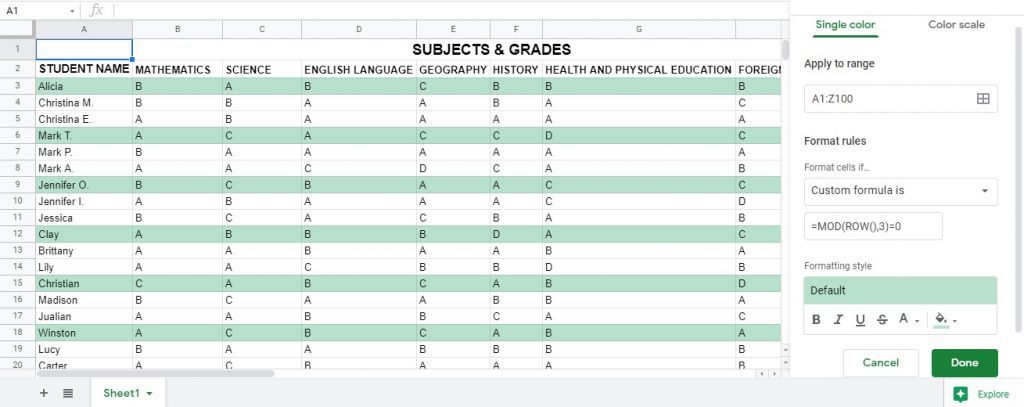
Follow the same steps as before but input =MOD(ROW(),3)=0 formula, instead. This will apply the conditional formatting to every third row in the sheet. To color every fourth row, just change the number 3 in the formula to 4.

You can use the same logic to color every 5th or 6th row, and so on.

You can also change 0 in the formula, so your formula will look like =MOD(ROW(),4)=3. This will color every fourth row, starting from the third one. So, instead of coloring rows 4, 8, 16, 20, etc, like before, our formula will now color rows 3, 7, 11, 15, etc.

How to Color Alternate Columns in Google Sheets (Conditional Formatting)

If you’d want to color alternate columns instead of alternate rows, you can do this by using the conditional formatting, as well. 

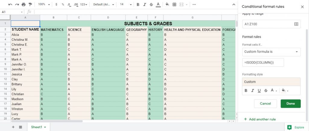
Open the sheet, access ‘Conditional formatting’, select a range, and input =ISEVEN(COLUMN()) as a custom formula. Select color and close the toolbar.

Just like we did with the rows, you can use the =ISODD(COLUMN()) formula to color the odd rows, too.

⚠️ A Few Notes About Coloring Alternate Rows or Columns in Google Sheets:

Here are a few simple notes you should know about coloring alternate rows or columns in Google Sheets:

• If any of the cells were already colored, the color will be overwritten once you use ‘Alternating colors‘ or ‘Conditional formatting‘ to color alternate rows. However, your original color settings won’t be lost. Once you remove the alternating colors, the previous color of the cell will appear again.
• When you insert new rows or columns in the formatted range, Google Sheets will automatically adjust the colors to match the alternate colors settings.
• If you insert new rows or columns before or after the formatted range, Google Sheets will also automatically apply the alternate colors settings.
• To apply the same conditional formatting to another range, you can use simple ‘copy‘ and ‘paste‘. Just make sure you select ‘Paste special > Paste conditional formatting only‘.

That’s all! Now you know how to color alternate rows in Google Sheets, as well as how to color every third or fourth row. And you’ve learned how to color alternate columns, too! Try it yourself, and see what you’ve learned today:

Apply conditional formatting along with a wide range of other Google Sheets formulas that will help you improve the readability of your sheet 🙂

Get emails from us about Google Sheets.

Our goal this year is to create lots of rich, bite-sized tutorials for Google Sheets users like you. If you liked this one, you'll love what we are working on! Readers receive ✨ early access ✨ to new content. There will be no spam and you can unsubscribe at any time.

Subscribe