


The EXACT function and comparison operators are useful when you need to compare two cells in Excel.
This guide will explain how you can compare two cells with and without case sensitivity.
Let’s look into a situation where you might need to determine whether two strings are equal.
Suppose you’ve received an invoice that contains a list of items purchased from a seller ordered in chronological order. Each item bought in the list comes with a specific item ID.
As the buyer, you’ve also kept track of your purchases by writing down the item IDs of each item bought. How can we determine whether your list and the seller’s invoice have the same items?
We can import both lists into the same spreadsheet using Excel. Both lists can be aligned such that each row should refer to the same item in the buyer’s list and seller’s list.
Afterward, we can use built-in functions in Excel to compare these two values. We can use the comparison operator ‘=’ if we want a case-insensitive comparison. If a case-sensitive comparison is required, we can use the EXACT function instead.
The EXACT function takes two strings as arguments. If the two strings are the same, the function will return TRUE. If the strings differ, EXACT returns FALSE.
Now that we know when to compare two cells in Excel, let’s see how we can use the previously mentioned methods on an actual spreadsheet.
A Real Example of a Sheet that Compares Two Cells in Excel
Let’s take a look at a real example of a spreadsheet that uses the Excel function to compare two cells in Excel.
In the example below, we have a table with three columns. The first and second columns hold the strings we want to compare to each other. The third column returns the result of that comparison.
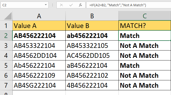
To get the values in Column C, we just need to use the following formula:
=IF(A2=B2; "Match";"Not A Match")
The formula above uses the equal sign. The character ‘=’ works as a comparison operator when placed between two values. The IF function returns custom text when a match is or isn’t found.
You can make your own copy of the spreadsheet above using the link attached below.
If you’re ready to try out these comparison functions in Excel, head over to the next section to learn how to do it yourself.
How to Compare Two Cells in Excel
This section will guide you through each step needed to start using Excel functions to compare two cells. You’ll learn how we can use the equal sign operator to perform case-insensitive comparisons. We’ll also show how the EXACT function performs case-sensitive comparisons between strings.
Follow these steps to start using these Excel functions:
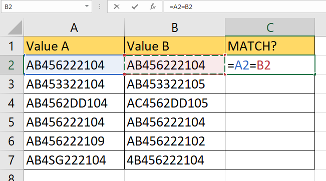
- First, select the cell we will use to compare our two values. In this example, we’ll start with the first cell in column C.

- Next, we can type the formula “=A=B” where A is the first value to compare and B is the second value to compare. Below, we’ve compared cells A2 and B2.
- Hit the Enter key to return the comparison result. In this example, we’ve found out that the strings in cells A2 and B2 are a match.
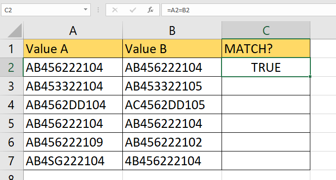
- Use the Fill Handle to apply the formula to the rest of the column.

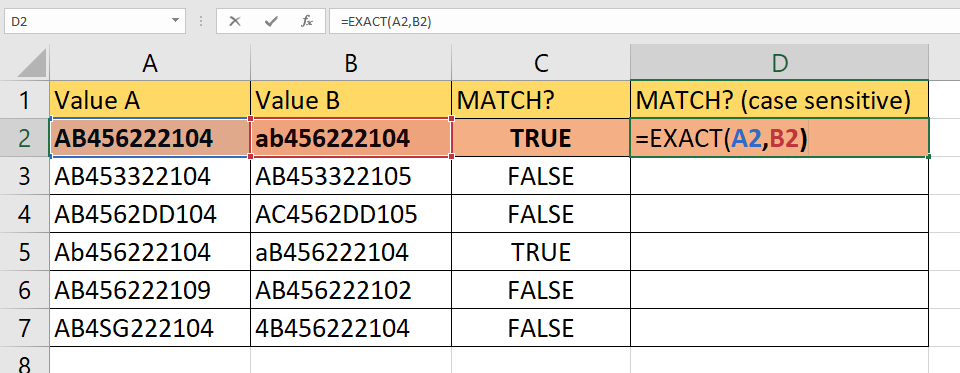
- If you want to use a case-sensitive comparison, we can use the
EXACTfunction. First, select the cell where you want to place our new formula.

- In this new cell, type in the
EXACTformula with the two values to compare as arguments.
- Hit the Enter key to return the result of the comparison. Afterward, use the Fill Handle to apply the
EXACTfunction to the rest of the column.

- To display text other than TRUE and FALSE, we can use an IF function. The first argument is our comparison formula. The second argument should be the string to display if the comparison is a match. The third argument refers to what is displayed if the two values do not match.
Frequently Asked Questions (FAQ)
- Can I use these methods on numerical data?
Both of these methods can be used on numerical data as well. However, comparisons will not consider any formatting changes made to the numerical data. For example, a number formatted as ‘$12,345.00’ will still be considered equal to the number formatted as ‘12345’ provided they are still numerical data. - How can I get a partial match?
If you want to compare characters based on a substring, you can use theLEFTorRIGHTfunction alongside our comparison methods. For example, if you want to compare the first five letters of both strings, you can use the formula=LEFT(A2, 5)=LEFT(B2, 5).
This step-by-step guide is everything you need to compare two cells in Excel. This article has shown how you can compare two strings using the EXACT function and the comparison operator ‘=’.
Comparing two strings for equality is just one example of a string operation that you can perform in Excel. With so many other Excel functions available, you can surely find one that suits your use case.
Are you interested in learning more about what Excel can do? Subscribe to our newsletter to find out about the latest Excel guides and tutorials from us.


