The Freeze panes feature in Excel is useful when you want a row or column always to be displayed when navigating your spreadsheet.
Freezing panes is especially useful if you have a header row that you want to be displayed even when the user scrolls vertically or horizontally.
Let’s take a look at a quick example of a scenario where we might consider using frozen rows and columns.
Suppose we have a table with a thousand entries. Each row includes information about a specific respondent in a survey. Most of the material provided are Yes or No questions, with the output placed as either 1 or 0.
Scrolling down the list, it may become difficult to read the table since we can no longer read the question corresponding to a given row. Similarly, if we continue navigating towards the right, it will become challenging to keep track of which respondent we are currently looking at.
Excel’s Freeze Panes feature allows users to “freeze” columns or rows in place to remain visible as the user navigates the spreadsheet.
Let’s learn how to freeze our own panes in Excel and take a look at some sample spreadsheets that use this feature.
A Real Example of Freezing Panes in Excel
Let’s take a look at a real example of a spreadsheet that uses the Freeze Panes feature.
The table below shows a list of employees from various companies around the globe. Since this list contains hundreds of entries, scrolling down will hide the header row. While it might be easy to differentiate the id column from the first_name column, it is possible that a user might not know whether a given value refers to a first name or last name.
In the spreadsheet below, we have frozen the first row so that the table’s header will be visible at all times.

You can make your own copy of the spreadsheet above using the link attached below.
If you’re ready to try out the Freeze Panes feature in Excel, move on to the next section to learn how to do it step by step.
How to Freeze Panes in Excel
This section will guide you through each step needed to start using the Freeze Panes feature in Excel. You’ll learn how we can use this feature to select rows and columns to freeze when navigating the spreadsheet.
Follow these simple steps to start using the Freeze Panes option in Excel:
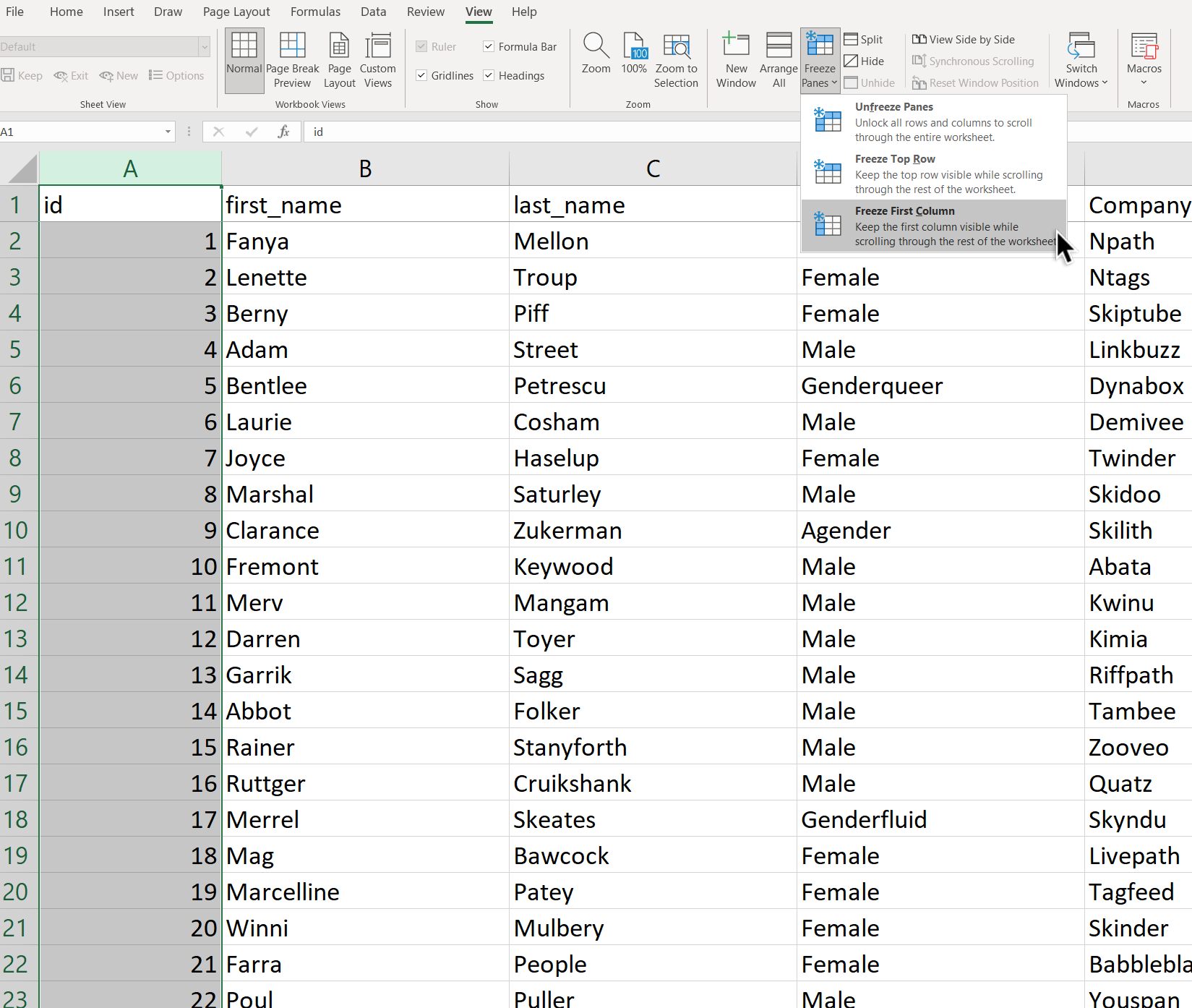
- First, we will try to freeze the first row. This is an important row since it contains our header. To do this, we must first select either the row itself or just cell A1.

- You can find the Freeze Panes feature in the View tab. Clicking on the icon will show us a dropdown menu with some options. Since we only want to freeze the top row, we can choose the Freeze Top Row option.

- The top row should now be frozen in place. While scrolling down, users should still see the table’s header.

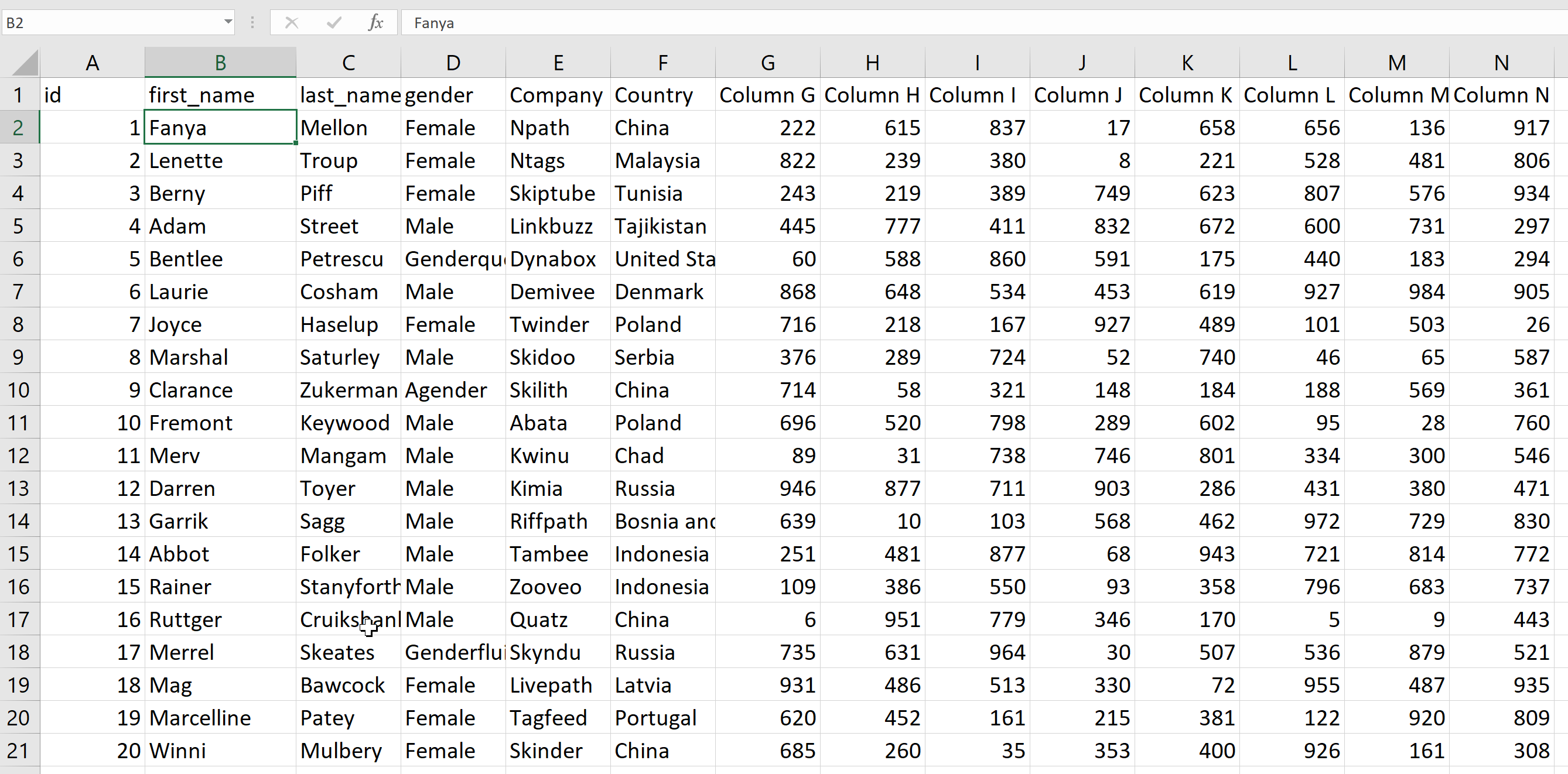
- If you want to freeze the first column instead, we can choose the Freeze First Column instead.
- Now that the first column is frozen, you can still see the id value even after scrolling further to the right of the sheet.

- If you want to freeze both rows and columns, you must select a specific cell. This cell must be just below the row you would like to freeze and just to the right of the column you would like to freeze. In the example below, choosing cell B2 will allow us to freeze both the first row and the second row.
If we were to choose cell C2 instead, we would freeze the first row and both Column A and Column B. - Once the target cell is selected, click on the Freeze Panes option. This is the first option under the Freeze Panes icon.

- Your spreadsheet should now have the specified number of rows and columns frozen.

- To unfreeze panes, select the Unfreeze Panes option under the Freeze Panes dropdown menu. This option will unlock all rows and columns in that particular sheet.

Frequently Asked Questions (FAQ)
- What is the difference between Freeze Panes and the Split feature?
The Split Panes feature splits the worksheet window vertically or horizontally. These Split Panes span the entire worksheet. We can use each of these panes to navigate our spreadsheet. The Freeze Panes feature still has only one pane where you can navigate, while a small portion of the cells is locked in place.
That’s all you need to remember to start using the Freeze Panes function in Excel. This step-by-step guide shows how easy it is to keep rows and columns visible even while scrolling.
The Freeze Panes is just one example of a useful feature you can use in Excel to make your spreadsheets easier to read and navigate. With so many other Excel functions out there, you can surely find one that suits your use case.
Are you interested in knowing more about what Excel can do? Subscribe to our newsletter to be the first to know about the latest guides and tutorials from us.