How to Perform a Kolmogorov-Smirnov Test in Excel

This guide will explain how to perform a Kolmogorov-Smirnov test in Excel.

We can use this test to determine if our sample data follows a normal distribution.

A normal distribution is a type of distribution that appears as a bell curve, with a symmetrical shape and most values falling close to the mean. Many statistical methods assume that data is normally distributed, so testing your dataset for normality is often a required step in statistics. 

To test for normality, statisticians perform calculations that will either support or reject the null hypothesis. This hypothesis states that the given distribution does not follow a normal distribution.

We can use the Kolmogorov-Smirnov test to test for normality. 

The Kolmogorov-Smirnov test, also known as the KS test, is a nonparametric test that allows you to determine if a sample follows a particular distribution.

Let’s look at a quick example where we might need to test for normality using a KS test.

Suppose you want to know if wind speed in a certain area follows a normal distribution. You obtain a sample dataset of 100 wind speed observations. 

We can perform the Kolmogorov-Smirnov test in an Excel sheet to determine how closely the sample follows a normal distribution. We will use the NORM.DIST function to compare the cumulative distribution of the sample with the expected normal distribution.

If the maximum observed difference is greater than a particular critical value, we can conclude that the sample does not follow a normal distribution.

Now that we know when to perform the Kolmogorov-Smirnov test in Excel, let’s learn how to use it and work on an actual sample spreadsheet.

A Real Example of Performing a Kolmogorov-Smirnov Test in Excel

The following section provides a sample problem where we can use the Kolmogorov-Smirnov test. We will also explain the formulas and tools used in these examples.

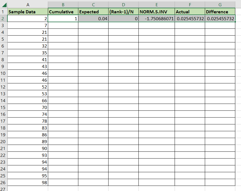
First, let’s take a look at our sample data. Our sample spreadsheet contains a table of 25 randomly-selected values from a larger population.

We’ll create multiple columns to find the maximum difference between the expected and actual cumulative distribution observed in the sample.

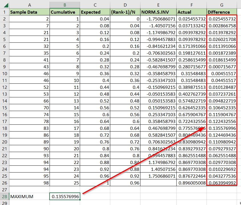
After finding the maximum difference, we’ll use a critical value lookup table to determine the results of the test.

For example, if we are using an alpha of 0.05 and a sample size of 25, then our critical value is 0.26404. Since the maximum difference is less than this critical value, we fail to reject the null hypothesis.

Do you want to take a closer look at our examples? You can make your own copy of the spreadsheet above using the link attached below. 

Use our sample spreadsheet to test out how we were able to generate each column.

If you’re interested in trying the Kolmogorov-Smirnov test in Excel, head over to the next section to read our step-by-step breakdown on how to do it!

How to Perform a Kolmogorov Smirnov Test in Excel

This section will guide you through each step needed to perform a Kolmogorov-Smirnov test in Excel. You’ll learn how to create each column needed to return the test statistic of the current sample data.

Follow these steps to perform a Kolmogorov-Smirnov test in Excel:

1. First, we’ll need to create multiple columns in our spreadsheet. Follow the column headers seen in the spreadsheet below.
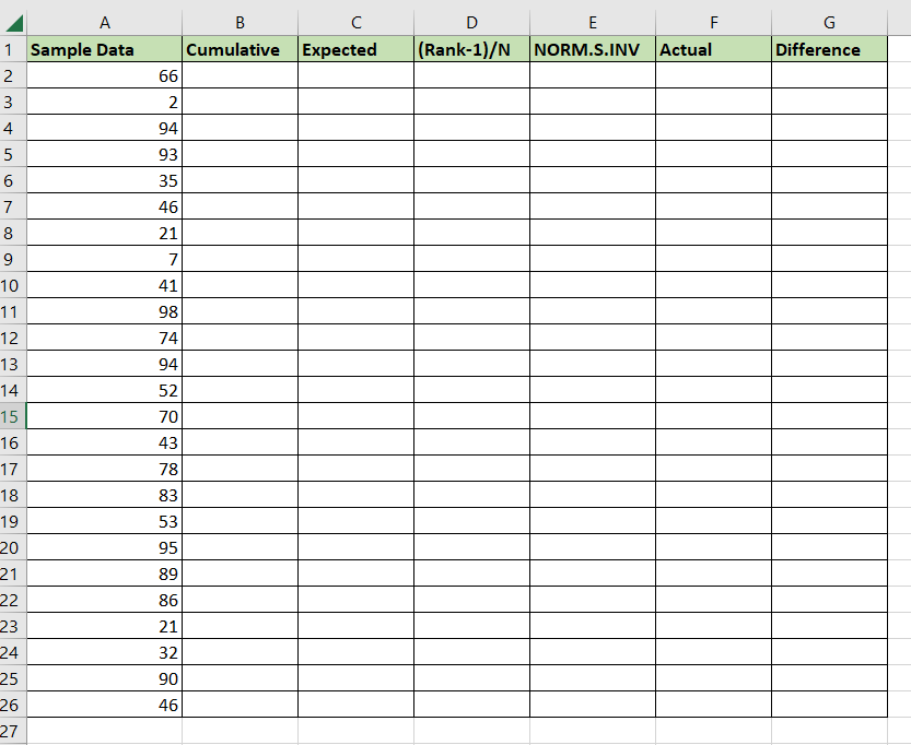   After adding the columns, ensure that the sample data is sorted in ascending order.
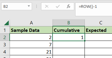
2. We’ll generate a cumulative count for the second column. We can subtract 1 from the current row number to enumerate each row. We can find the current row number by calling the ROW function.
   
3. Next, we’ll divide the cumulative row count by the sample size. We can calculate the sample size by using the COUNT function.
   
4. Next, we’ll use the formula =(B2-1)/COUNT($A$2:$A$26) to fill the fourth column.
   
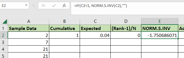
5. We’ll input the expected value as an argument for NORM.S.INV.
   
6. Next, we’ll find the actual cumulative probability of the current data point using the NORM.DIST function. We’ll use the AVERAGE and STDEV.S functions to calculate the mean and standard deviation of the sample data.
   
7. We’ll fill the last column with the absolute difference between columns F and D. We’ll use the ABS function to convert our difference into an absolute value.
   
8. Select the cell range B2:G2 and use the Fill Handle option to fill out the rest of the table.
   
9. You should now have a complete table of values for the KS test.
   
10. Use the MAX function on the column labeled ‘Difference’ to get the largest value in the range. We can compare the maximum value with the appropriate critical value to determine if we can reject the null hypothesis.
    

These are all the steps you need to perform the Kolmogorov-Smirnov test in Excel.

This step-by-step guide should provide you with all the information you need to use the Kolmogorov-Smirnov test in Excel.

This test is just one example of the many statistical methods you can use in your spreadsheets. Our website offers hundreds of other functions and methods to help you get more out of Microsoft Excel.

With so many other Excel functions available, you can find one appropriate for your use case.

Don’t miss out on our team’s new spreadsheet tips, tricks, and best practices. Subscribe to our newsletter to stay updated on the latest guides from us!

Get emails from us about Excel.

Our goal this year is to create lots of rich, bite-sized tutorials for Excel users like you. If you liked this one, you'd love what we are working on! Readers receive ✨ early access ✨ to new content.

Subscribe