This guide will explain how to populate a list based on cell values in Excel.
The user can follow our methods to add values to lists quickly and easily based on other cells in the spreadsheet. This can be helpful when organizing data or creating reports.
In this article, we will go over two methods that can populate a list: data validation and the FILTER function.
Drop-down list data validation allows you to create a list of valid values that can be selected from a drop-down menu. This can be helpful when you want to restrict the values that can be entered into a cell.
Later, we will explain how we can set up two drop-down lists where the values shown in the second are dependent on what the user selected on the first drop-down list.
We can also use the FILTER function to populate a list based on cell values. The FILTER function allows you to filter a range of data based on the criteria that you specify. This can be helpful when you want to view a subset of data that meets certain criteria.
Let’s take a look at an actual sample spreadsheet that populates a list based on a cell value.
A Real Example of Populating a List Based on Cell Value
The following section provides several examples of how to populate a list based on cell values. We will also go into detail about the formulas and tools used in these examples.
Populating a List Using the FILTER Function
First, let’s take a look at a real example of the FILTER function populating a list in Excel.
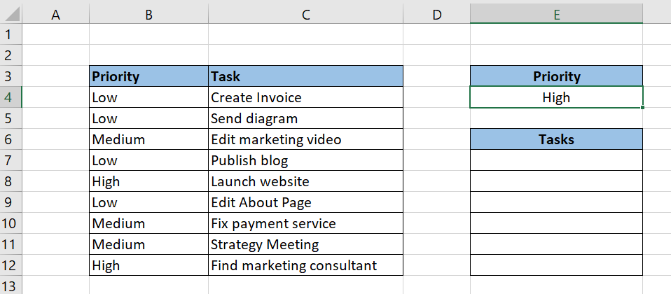
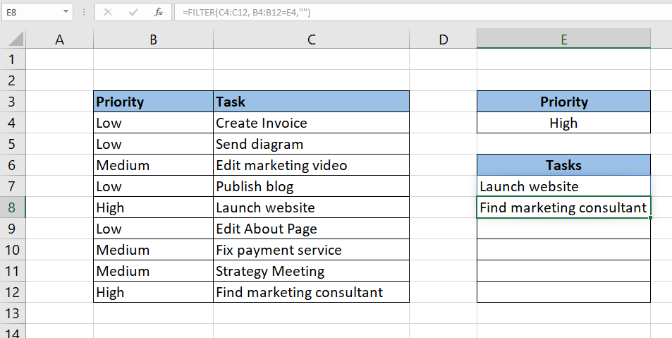
In the spreadsheet below, we have a list of tasks and their corresponding priority. The spreadsheet includes the functionality to filter this table based on the indicated priority in cell E4.

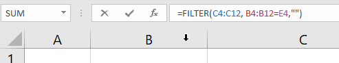
To get the values seen in the range starting at E7, we can use the following formula:
=FILTER(C3:C11, B3:B11=E3,"")
If we change the value in cell E4, the output of our FILTER function will also change.

Populating Drop-down Lists
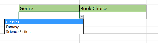
In this example, we have several books from different genres of literature.
We can help the user narrow down a book choice by providing two drop-down menus.
The first drop-down menu will provide the following choices: Classics, Fantasy, and Science_Fiction.
We want to populate our second drop-down list. With books based on what the user selected in the first drop-down list.

We can use the INDIRECT formula to control which range of books appear in the second drop-down list.
Do you want to take a closer look at our examples? You can make your own copy of the spreadsheet above using the link attached below.
Use our sample spreadsheet to test out both methods we’ve shown in this section.
If you’re ready to try populating a list based on cell value, head over to the next section and read our step-by-step tutorial on how to do it!
How to Populate a List Based on Cell Value in Excel
This section will guide you through each step needed to start populating a list based on a given cell value in Excel.
You’ll learn how to apply the FILTER function to a range to output entries that follow a certain criteria. We will also explain how to populate a drop-down list conditionally using the INDIRECT function.
Follow these steps to start populating a list based on cell value in Excel:
- First, determine the cell that will control what values to populate. In this example, we will set cell E4 as our basis for populating the empty range in the range E7:E12.
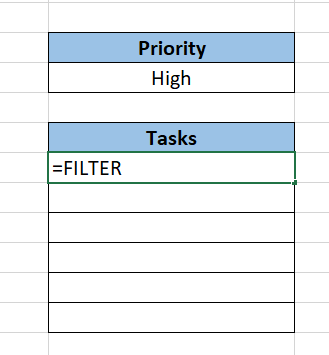
- In the first cell of the empty range, type ‘=FILTER’ to start the
FILTERfunction.
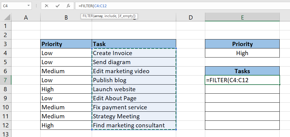
- The
FILTERfunction’s first argument determines the range to use when returning filtered values. In this example, we’ll return a filtered subset of values from the range C4:C12.
- Next, we must write the conditional statement that will decide which entries to filter out. We wrote the conditional statement
E4=B3:B12to ensure that the function only prints out tasks with a priority equal to what is written in cell E4.

- We can use the optional third argument to set what to output when the function returns an empty array. In this example, we’ll return an empty string.
- Hit the Enter key to evaluate the
FILTERfunction.
After following these instructions, you should have an idea of how to populate a range with the FILTER function.
Next, let’s look into how to populate a drop-down list in Excel. We will set up two drop-down lists that will help the user select a book from a database.
- First, select the cell that will hold the first drop-down menu. In this example, we’ll add a drop-down list in cell B22.

- In the Data Validation pop-up, provide the range that includes the genres to filter with.

- You should now have a cell with drop-down list data validation.
- Next, we’ll have to add names to each column in our data. Select the source range and click on the Create from Selection option in the Formulas tab

- In the dialog box, check the option labeled ‘Top row’. This will ensure that we can use the top row of our selection to refer to each column individually.

- Next, we’ll create another drop-down list using data validation. Instead of selecting from a predetermined range, we’ll use the
INDIRECTfunction to refer to the ranges we’ve named in the previous steps.

- The second drop-down list should now be populated with different values based on what genre the user chose in the first drop-down list.
These are all the steps you need to follow to populate a list based on cell value.
This step-by-step guide is a quick introduction to populating a list based on cell values in Microsoft Excel. Populating lists using data validation and Excel functions allows your spreadsheet to become more dynamic.
Our website offers hundreds of other functions and methods to help you get more out of Microsoft Excel. With so many other Excel functions available, you can find one appropriate for your use case.
Don’t miss out on our team’s new spreadsheet guides and best practices. Subscribe to our newsletter to stay updated on the latest guides from us!