Knowing how to separate the first and last name in Google Sheets is useful if you want to split the given names into first and last names.
Meaning, the function can be used to split names up by first and last name, if you have the list of full names in one column.
Table of Contents
In this article, we will be discussing the 3 convenient ways of separating the first and last names in Google Sheets:
- Using the SPLIT function
- Using the Split text to columns feature in the Data menu of Google Sheets
- Using the Text functions (RIGHT, LEFT, LEN, FIND functions)
The rules for separating the first and last name in Google Sheets are as follows:
- In this article, we will only be focusing on names with neatly two parts: first and last name.
- For names, which are composed of other than first and last names, will be discussed in a separate article. So be sure to subscribe to be notified.
- The results of separating first and last names using the SPLIT function are dynamic, which means that any changes in the cell that’s a reference to the first argument of the function will reflect automatically in the resulting values.
- The results of separating first and last names using the Split text to columns feature are static. The method would alter or overwrite the values of the given list of full names.
Let’s take an example.
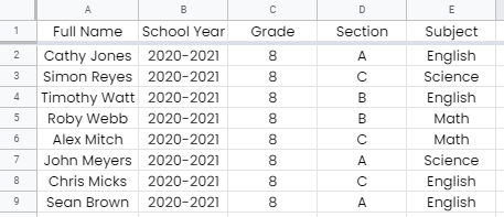
Rick, a teacher in grade school, created a Google Form for his attendance tracker of his students. Below are his students’ form responses:
Now, he’d like to add a new column that separates the first and last name in Column A. Using the SPLIT function, he was able to come up with the results below:
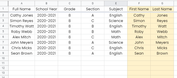
He put the SPLIT function inside the ARRAYFORMULA function so that whenever a new entry is submitted, the full name gets sliced automatically into first and last name in Column F and G, respectively.
Clever, right?
Let’s have another example!
Jackie owns a few websites and has been trying to track her subscribers. She was planning to send each of her subscribers a personalized message to thank them for their support. Using a script, she will be able to attain her goal. What she needs is to extract the first name from the list of full names of her subscribers. See below her list of subscribers:

Jackie has been an avid fan of Sheetaki website and learned a bunch of functions. Using a combination of the Text functions, she was able to extract the first names from the given full names of her subscribers:

Watch out for a more advanced tutorial and examples on how you separate the first and last names in the coming weeks. Be sure to subscribe to be notified.
Awesome! Let’s begin getting to know more about the process and steps in separating first and last names in Google Sheets.
The Anatomy of the SPLIT Function, Split Text to Columns Feature, and Text Functions used for Separating the First and Last Name
In this article, we will be focusing more on the method and procedures in separating the first and last name. For more information and examples about the functions that we are about to use, please visit the previous articles by clicking on the links provided below.
The syntax (the way we write) of each of the functions is as follows:
=SPLIT(text, delimiter, split_by_each, remove_empty_text)
=FIND(search_for, text_to_search, [starting_at])
=LEFT(string, [number_of_characters])
=RIGHT(string, [number_of_characters])
=LEN(text)
To dissect each function, their arguments and understand what each of these terms means, feel free to refer to the links below:
Also, you may want to visit the article regarding the feature Split text to columns, which we’ve already tackled in our previous post.
A Real Example of Separating First and Last Name
Take a look at our form responses example below to see how to separate first and last name in Google Sheets:

In the example above, we used the SPLIT function method to separate the first and last names. The function splits the full names in Column A into first and last names in Column F and G, respectively.
The function has two arguments. One is the text to split and the other one is the delimiter, which tells the function where to split.
We all know that the full name is composed of first and last name, separated by the space. So, it’s easy for the SPLIT function to do the slicing of data.
The results of the SPLIT function are dynamic, which means that any changes to the data in the cell address of the first argument will reflect in the resulting values.
On the other hand, the results of the Split text to columns feature are static. Please see our example below:

Once you pick the delimiter, the split results will overwrite our given full names:

The Split text to columns is a preferred method when you want to split the text once or twice. Otherwise, it’s best to use a formula, if you want to split the given text values multiple times or repeatedly.
What if you only want to extract a certain part of the given text? In this case, you only want to get the first name in the given list of full names.
Yes, you may still use the SPLIT function. However, since you’d only need the first name, you have to do extra steps to delete the last name, which is less efficient in this scenario.
This is when the combination of Text functions is preferable.
See our sample below:
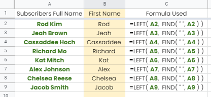
In the example above, notice that we used two Text functions, the LEFT and FIND function. Let’s dissect each function’s role to our goal here.
First, we all know that the character that separates the first and last name is the space character “ “. This character identifies the end of the first name. So, we would ask our formula to find its position from the given text values.

Check that we used the FIND function, which returns the position at which a string is found within the text. In this case, we are looking for the position of the character space “ “, which is the first argument of our FIND function, in the full name value, which is the second argument.
It returns the number 4, which means space is the fourth character in the “Rod Kim” text value.
Now that we already found the position of the character space “ “, let’s now ask Google Sheet to return us the first name only from our given text value.

Notice the second Text function that we used to get the first name, the LEFT function, which returns a substring from the beginning of a specified string.
We told Google Sheet to return us the characters, first up to the fourth one, from the left in the given text value “Rod Kim”. That’s basically ‘R’ as the first character, ‘o’ is the second one, ‘d’ is the third one, and finally space “ “ as the fourth character.
Since our formula includes the space “ “, or the last character, as the return value, what we can do is subtract 1 from the FIND function part. This means that we only need 3 as the return value of our FIND function, instead of 4. Hence, we will always subtract 1 from the result. So the final formula should be:

In our last example below, we will show you how to extract the last name in the given list of full names.

Since we were able to retrieve the first name using the FIND and LEFT function, extracting the last name should be easy.
We know that the formula in finding the space “ “ is =FIND( ” “, A2 ). We can use this formula as well in finding what’s left of the characters in the given text values. Subtracting this formula from the total number of characters of the given text values would give you the remaining characters after space “ “.

The LEN function returns the length or the number of characters of a given string. In this case, =LEN (A2) would return 7, which is the exact count of characters in the text “Rod Kim”.
Subtracting the result of =FIND(“ “, A2) from that would give you 3, which tells us that there are only 3 characters after space.
This number is what we can use to retrieve the last name in the text value “Rod Kim”.

Using the RIGHT Function, which returns a substring from the end of a string, and the combination of the LEN and FIND functions, we can retrieve the last name in the given full name.
We passed two arguments in the RIGHT function, one is the given text value, and the second one is the number that tells us what’s left after the space from the left, which is 3.
The RIGHT function returns the characters up to the 3rd one from the right of the given text value. These characters are ‘K’, ‘i’, and ‘m’, which is the last name in the given text value.
You may make a copy of the spreadsheet using the link I have attached below.
How to Separate First and Last Name in Google Sheets
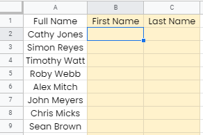
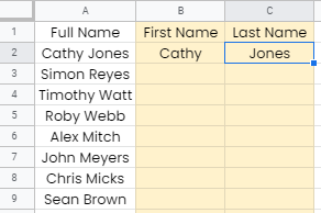
- Simply click on any cell to make it the active cell. For this guide, I will be selecting B2, where I want to show my result. This means that cell C2 will hold the value for the last name.
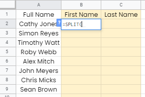
- Next, type the equal sign ‘=‘ to begin the function and then follow it with the name of the function, which is our ‘split‘ (or ‘SPLIT‘, not case sensitive).
- Type open parenthesis ‘(‘ or simply hit Tab key to let you use that function.
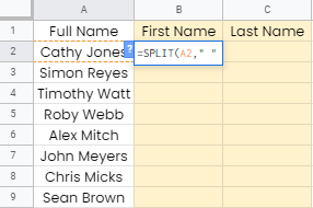
- Now the fun part! Let’s give our function the first argument, which is the text value. Type in A2.

- To let the Google sheet know that we’re done typing our first argument, we should now type in the delimiter or the character that separates each argument on a function. In this case, type comma ‘,’ followed by the second argument, which is the space “ “.
- Finally, just hit your Enter or Tab key. The cells B2 and C2 will now show you the first and last name, respectively.
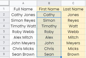
- Copy the formula down to the remaining rows. Columns B and C will now show you the results of the SPLIT function.
- Alternatively, we can use the Split text to columns feature in the Data menu of Google Sheets.
- Make your entire list active by clicking on it.
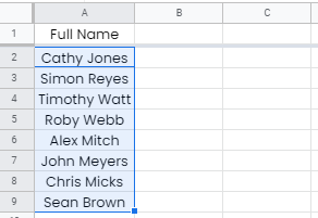
- Click Data in menu options, then Split text to columns.

- Now, in the Separator selector, pick the delimiter Space.
- Column A will be altered with the results of the process and Column B will hold the last name values.
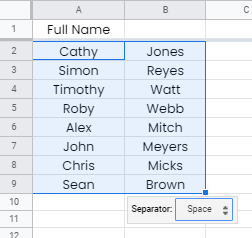
- Lastly, change the header title, accordingly.
That’s pretty much it. You can now separate first and last names in Google Sheets together with the other numerous Google Sheets formulas to create even more powerful formulas that can make your life much easier.