This guide will explain how you can use the FILTER function to use VLOOKUP on only checkbox-checked rows in Google Sheets.
We can use the FILTER function to return a set of rows that meet specific conditions. In this case, we’ll use the function to select rows with a corresponding checked checkbox.
Let’s take a look at a quick example where we can use the FILTER and VLOOKUP functions together.
Suppose you have a spreadsheet with data for a list of available talks and seminars. You’ve set up the sheet so that the user can search for the event they want to participate in. To facilitate the search, you’ve added several VLOOKUP formulas to fill in certain details based on the search string input.
Since some events get canceled or run out of slots, you’ve added another column to your dataset that holds a checkbox. Is it possible to modify your VLOOKUP function so that only events with a checkbox appear
With the FILTER function, we can output a range that only returns rows that meet certain criteria. In this case, if the checkbox column is left unchecked, that row will be filtered out.
The IF function is another function we can use to achieve the same effect. In the next section, we will explain how to set up a modified VLOOKUP with both functions.
Now that we know when you might need to use VLOOKUP for checkbox-checked rows, let’s take a look at some sample spreadsheets.
A Real Example of Using VLOOKUP for Checkbox Checked Rows
Let’s take a look at a real example of a selective VLOOKUP function being used in a Google Sheets spreadsheet.
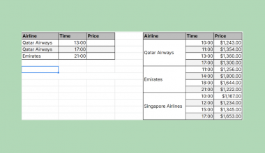
In this case, we have a lookup table containing details on specific classes. The last column of the lookup table indicates whether the class is available or not. The sheet owner can easily mark it available or unavailable through a checkbox.

Cells G4 and G5 return details of a specific class specified in cell G3. These cells will return a #N/A error if the class is unavailable.

To get the values in cells G4 and G5, we just need to use the following formula:
=VLOOKUP(G2,FILTER(A3:D15,D3:D15),3,0)
The first argument of the VLOOKUP function is our lookup value. In this example, we’re prompting the user to write down the class they want to find details for. The second argument is the table array. Our formula uses the FILTER function to return an array consisting of rows with a checked checkbox.
The third argument indicates which row of the table array to output. In the formula above, we indicated the third row to return the end time of the class. We place ‘0’ in the final argument to indicate that our lookup table does not contain sorted data.
Alternatively, we can also use the IF function to filter out the lookup table.
=VLOOKUP(G2,IF(D3:D15,A3:C15),2,0)
You can make your own copy of the spreadsheet above using the link attached below.
If you’re ready to try out the selective VLOOKUP function in Google Sheets, let’s start writing it ourselves!
How to Use VLOOKUP in Checkbox Checked Rows in Google Sheets
This section will guide you through each step needed to start using the FILTER function to lookup from a select number of rows in Google Sheets. You’ll learn how we can modify the VLOOKUP formula to only lookup values in rows where the checkbox is checked.
Follow these steps to start using the modified VLOOKUP function:
- First, locate the dataset you want to use as a lookup table. Add a new column and fill that new column with checkboxes.

- Next, use the checkboxes to select the rows you want to include when using the lookup table. In this example, we select all classes in the table that still have slots for interested students.

- We will now add three additional cells. The first shaded cell below will act as our search bar. The user will enter their desired class in this cell. Next, we’ve added two more cells that will use our modified
VLOOKUPformula to pull up the indicated class’s start and end time.

- Next, we’ll add the
VLOOKUPformula to look up the start time of the class indicated in cell G2. TheVLOOKUPformula uses theFILTERfunction to use column D as a filter for column B.

- We will do the same for cell G5. The
FILTERfunction will filter out column C using the checkboxes in column D.

- Instead of using the
FILTERfunction, we can also use theIFfunction to filter out our lookup table when usingVLOOKUP.

This step-by-step guide should be all you need to start using VLOOKUP in a subset of rows in Google Sheets. Our guide shows how easy it is to use the FILTER and IF function to only select cells that have been marked with a check.
The FILTER and VLOOKUP functions are both powerful functions you can use in Google Sheets to interact with your data. With so many other Google Sheets functions available, you can surely find one that works best for you.
Are you interested in learning more about what Google Sheets can do? Do subscribe to our Google Sheets newsletter to keep up with the latest guides and tutorials from us.