The HYPERLINK function in Google Sheets is useful if you want to create a clickable hyperlink with a formula.
Meaning, the HYPERLINK function returns a hyperlink from a given destination and link text.
Table of Contents
The rules for using the HYPERLINK function in Google Sheets are as follows:
- The first argument, or the link_location, should be passed as a text string enclosed with quotation marks or a cell reference that contains the link path as text.
- If the second argument, which is the friendly_name, is not provided, the HYPERLINK function will display link_location as the friendly_name.
- To select a cell that contains the HYPERLINK function without following the link, use arrow keys or right-click the cell.
Let’s take an example.
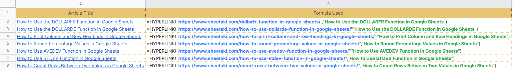
Rod is a writer at Sheetaki.com. He created a file in Google Sheet with all the articles he has written and published.

He wants to reorganize the table in such a way that each article title would be a hyperlink to the published article.
How else could he execute such a setting?
Well, that’s where our HYPERLINK function will come in handy.
Rod used the HYPERLINK function to create a clickable hyperlink which is linked to each of the published articles in Sheetaki.com

He no longer needed the second column, which is where the links of published articles were located.
Pretty convenient, right?
Watch out for a more advanced tutorial and examples on how you can use the HYPERLINK function in the coming weeks. Be sure to subscribe to be notified.
Awesome! Let’s begin getting to know more about our HYPERLINK function in Google Sheets.
The Anatomy of the HYPERLINK Function
So the syntax (the way we write) of the HYPERLINK function is as follows:
=HYPERLINK(link_location, [friendly_name])
Let’s dissect this thing and understand what each of these terms means:
- = the equal sign is just how we start any function in Google Sheets. It is how Google Sheets understand that we are asking it to either do computation or use a function.
- HYPERLINK() this is our HYPERLINK function. It returns a clickable hyperlink.
- link_location is the path to the file or page that needs to be opened.
- [friendly_name] is an optional argument. It is the link text to display in a cell.
A Real Example of Using HYPERLINK Function
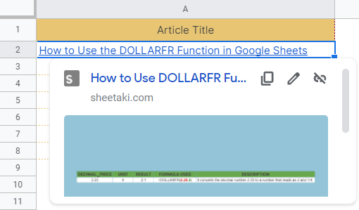
Let’s take a look at the new version of Rod’s table below to see how the HYPERLINK function is used in Google Sheets.
Rod was able to convert the article titles into hyperlinks which will open the published article once clicked.
The HYPERLINK function is pretty much straightforward. You have a link that you want to put in a text? Go ahead and pass it to the HYPERLINK function and see the magic happens.
What makes it straightforward?
Well, the HYPERLINK function only needs two arguments to do its job. The first one is the link_location, which is the path to the file or page that you’d like to open.
In the example above, the first link_location used is the link to the published article.

The second argument is the friendly_name, which is the link text to be displayed in a cell. It is the friendly_name that holds the link of the page that will be opened.
In the example above, the friendly_name used is the title of the article.

The result of the HYPERLINK function, in this case, is the friendly_name with the link in it.

Note that the friendly_name is an optional argument. This means that even if it’s not supplied in the HYPERLINK function, it will not return an error message.
However, the function will display link_location as the friendly_name.

So when Rod likes to visit the published article, he only needs to click on the cell to open the page.
You may make a copy of the spreadsheet using the link I have attached below.
How to Use HYPERLINK Function in Google Sheets
- Click on any cell to make it the active cell. For this guide, I will be selecting A2, where I want to show the result.

- Next, type the equal sign ‘=‘ to begin the function and then follow it with the name of the function, which is our ‘hyperlink‘ (or ‘HYPERLINK‘, not case sensitive like our other functions).

- Type open parenthesis ‘(‘ or simply hit Tab key to let you use that function.

- Now the exciting part! Let’s give our function its first argument, the link_location. You can pass a cell address that contains the URL. Alternatively, you can directly pass the URL. In this example, I will provide the direct URL to our HYPERLINK function. Type in ‘https://www.sheetaki.com/dollarfr-function-in-google-sheets/’. Don’t forget to enclose it with quotation marks (“”).

- To let the Google sheet know that we’re done typing our first argument, we should now type in the delimiter or the character that separates each argument on a function. In this case, type comma ‘,’.

- Type in our second argument, which is the friendly_name. Similar to the first argument, you may use a cell address that contains the friendly_name or you can directly pass the string to the HYPERLINK function. In this case, we will pass the title directly. Type in ‘How to Use the DOLLARFR Function in Google Sheets’. Don’t forget to enclose it with quotation marks (“”).

- Finally, hit your Enter or Tab key. Cell A2 will now show you the return value of the HYPERLINK function, which is the hyperlinked title of the article.
- Apply the same process to other titles with their corresponding published articles.
That’s pretty much it. You can now use the HYPERLINK function in Google Sheets together with the other numerous Google Sheets formulas to create even more powerful formulas that can make your life much easier.