This guide will explain how you can use the SUMPRODUCT function with merged cells in Google Sheets.
We’ll show you how you can unmerge the cells during the computation process using a Google Sheets formula.
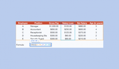
The SUMPRODUCT function can multiply multiple arrays together to return the sum of products. For example, let’s say you have a table of items for sale. Each item has a number indicating the quantity in stock and another number indicating its price. We can get the sum of products of these two ranges to get the total value of the items in stock.
Users may encounter an issue trying to use the SUMPRODUCT function when your ranges include merged cells.
SUMPRODUCT will only consider the first cell when handling merged cells. All other cells that were combined to form the merged cell will receive a value of 0. This may lead to an inaccurate result.
If we want to use the merged cells correctly, we will have to unmerge them somehow.
If we unmerge them using the built-in Unmerge option, we’ll be left with several blank cells. This is because only the first cell of the unmerged selection will retain the merged cell’s value.
We can either fill in the blanks manually or use a formula to create a modified copy of the original values dynamically.
Since we know what we need to do to make the SUMPRODUCT function work with merged cells, let’s look into a spreadsheet that solves this issue.
A Real Example of Using SUMPRODUCT with Merged Cells in Google Sheets
Let’s take a look at a real example of how we can use the SUMPRODUCT function on a spreadsheet with merged cells.
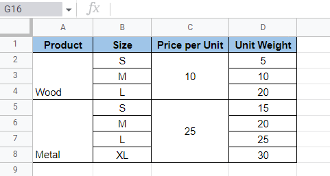
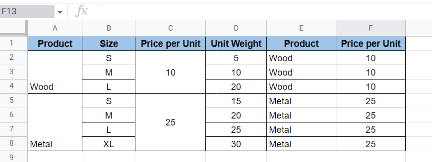
Suppose you have a business that sells storage boxes. You offer two types of products: wood and metal. For each of these types, you also offer Small, Medium, and Large sizes. Each combination of type and size has a different weight. You compute the item price by multiplying the weight by the price per unit of weight.
To compute the price, we can use the SUMPRODUCT function. However, we must first handle the merged cells.
In the example below, we added helper columns E and F to make it easier to use the SUMPRODUCT function.

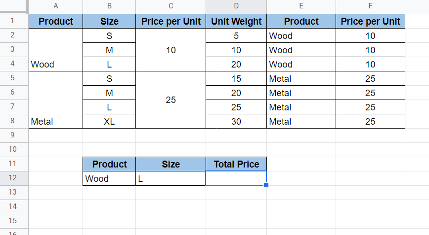
To get the result in cell D12, we just need to use the following formula:
=SUMPRODUCT(G2:G8=B12,B2:B8=C12,D2:D8,H2:H8)
Our first two arguments help filter out which rows we want to include. Since row 4 is the only row that outputs TRUE on both arguments, SUMPRODUCT will multiply D20 and F10 automatically. This gives us a final price of $200.
You can make your own copy of the spreadsheet above using the link attached below.
If you’re ready to try out the SUMPRODUCT function in Google Sheets, let’s begin writing it ourselves!
How to Use SUMPRODUCT with Merged Cells in Google Sheets
This section will guide you through each step needed to use the SUMPRODUCT function with merged cells in Google Sheets. You’ll learn how we can use a simple IF formula to split merged cells into individual cells with duplicate values. Afterwards, we’ll use the SUMPRODUCT function to determine the price of an item of a given type and size.
Follow these steps to start using the SUMPRODUCT function:
- First, we’ll show you the manual method for converting merged cells into a workable range for
SUMPRODUCT. Select the columns that have merged cells. Type Ctrl+C to copy the selected cells.

- Next, we’ll paste the selected columns as new columns in our table.

- While these cells are still selected, select the Unmerge option in the Merge cells dropdown menu.
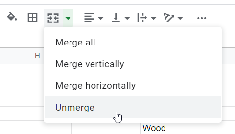
- The selected cells should now be converted to individual cells. The cell values should now only remain in the first cell of each formerly merged cell.

- Using the Fill Handle tool, we can fill out the empty spaces in the modified columns manually.
- If using the Fill Handle tool is impractical, we can use a formula to populate our new fields dynamically. Ensure that the value you’re comparing to 0 is in the same column as the original value. In cell E2, we’ve added the formula
IF(A2=0, E1, A2).

- Use the Fill Handle tool to populate the entire column.

- Afterwards, perform this same technique on all helper columns.

- Now that we’ve populated our helper columns, we can now use the
SUMPRODUCTfunction to compute prices. In this example, we want to get the price of a product given the information provided in cells B12 and C12.
- In our
SUMPRODUCTfunction, we’ll need four arguments to determine the price. The first argument compares our product range with the target product. The second argument does the same but with sizes. Our last two arguments will multiply the price range with the unit weight range.

- Once you hit the Enter key, Google Sheets will evaluate the
SUMPRODUCTfunction. In this example, we’ve determined at last that the price of our Wood product of size L is $200.
This step-by-step guide should be all you need to start using SUMPRODUCT on a dataset with merged cells. In conclusion, a simple IF formula can convert merged cells into individual cells with duplicate values.
The SUMPRODUCT function is just one example of a mathematical function in Google Sheets. With so many other Google Sheets functions available, you can surely find one that suits your use case.
Are you interested in learning more about what Google Sheets can do? Subscribe to our newsletter to find out about the latest Google Sheets guides and tutorials from us.